- Efficient Inference in Fully Connected CRFs with Gaussian Edge Potentials, P. Krähenbühl, V. Koltun
- Fast and Accurate k-means For Large Datasets, M. Shindler, A. Wong, A. Meyerson
- Hashing Algorithms for Large-Scale Learning, P. Li, A. Shrivastava, J. Moore, A. König
- Hogwild: A Lock-Free Approach to Parallelizing Stochastic Gradient Descent, B. Recht, C. Re, S. Wright, F. Niu
- Generalizing from Several Related Classification Tasks to a New Unlabeled Sample, G. Blanchard, G. Lee, C. Scott
- How biased are maximum entropy models? J. Macke, I. Murray, P. Latham
- On Tracking The Partition Function, G. Desjardins, A. Courville, Y. Bengio
- Selecting Receptive Fields in Deep Networks, A. Coates, A. Ng
- Shallow vs. Deep Sum-Product Networks, O. Delalleau, Y. Bengio
- Statistical Tests for Optimization Efficiency, L. Boyles, A. Korattikara, D. Ramanan, M. Welling
Monday, November 21, 2011
Interesting papers coming up at NIPS'11
There's a number of accepted papers whose camera-ready versions have been posted already. Here are the ones I found interesting. I'll give further update on these after the conference.
Sunday, November 13, 2011
Shapecatcher
Here's a cool tool I stumbled across reading John Cook's blog -- Shape Catcher looks up Unicode value from a drawing of a character.
Apparently it uses Shape Context features.
This motivated me to put together another dataset, unlike notMNIST this focuses on the tail end of Unicode, this is 370k bitmaps representing 29k Unicode values, grouped by Unicode
Apparently it uses Shape Context features.
This motivated me to put together another dataset, unlike notMNIST this focuses on the tail end of Unicode, this is 370k bitmaps representing 29k Unicode values, grouped by Unicode
Wednesday, November 09, 2011
Google1000 dataset
This is a dataset of scans of 1000 public domain books that was released to the public at ICDAR 2007.
At the time there was no public serving infrastructure, so few people actually got the 120GB dataset.
It has since been hosted on Google Cloud Storage and made available for public download
To download it, ie, with Python on Linux box
- http://commondatastorage.googleapis.com/books/icdar2007/README.txt
- http://commondatastorage.googleapis.com/books/icdar2007/[filename]
- [filename] goes from Volume_0000.zip to Volume_0999.zip
To download it, ie, with Python on Linux box
import os
for i in range(1000):
 if count>1: break
 fname = 'Volume_%04d.zip'%(i)
 f = 'curl -L http://commondatastorage.googleapis.com/books/icdar2007/%s -o %s'%(fname,fname)
 os.system(f)
The goal of this dataset is to facilitate research into image post-processing and accurate OCR for scanned books.
Sunday, November 06, 2011
b-matching as improvement of kNN
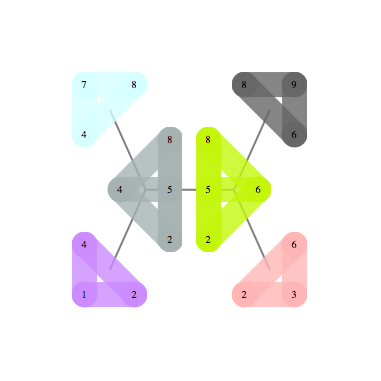
Below is an illustration of b-matching from (Huang,Jebara AISTATS 2007) paper. You start with a weighted graph and the goal is to connect each v to k u's to minimize total edge cost. If v's represent labelled datapoints, u's unlabeled and weights correspond to distances, this works as a robust version of kNN classifier (k=2 in the picture) because it prevents any datapoint from exhibiting too much influence.
They show that this restriction significantly improves robustness to changes in distribution between training and test set. See Figure 7 in that paper for an example with MNIST digits.
This is just one of a series of intriguing papers on matchings that came out of Tony Jebara's lab, there's a nice overview on his page that ties them together.
Tuesday, October 25, 2011
Google Internship in Vision/ML
My group has intern openings for winter and summer. Winter may be too late (but if you really want winter, ping me and I'll find out feasibility). We use OCR for Google Books, frames from YouTube videos, spam images, unreadable PDFs encountered by the crawler, images from Google's StreetView cameras, Android and few other areas. Recognizing individual character candidates is a key step in OCR system. One that machines are not very good at. Even with 0 context, humans are better. This shall not stand!
For example, when I showed the picture below to my Taiwanese coworker he immediately said that these were multiple instance of Chinese "one".

Here are 4 of those images close-up. Classical OCR approaches, have trouble with these characters.
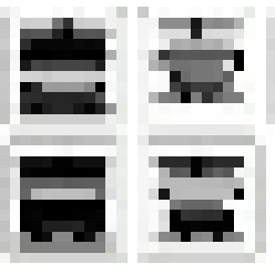
This is a common problem for high-noise domain like camera pictures and digital text rasterized at low resolution. Some results suggest that techniques from Machine Vision can help.
For low-noise domains like Google Books and broken PDF indexing, shortcomings of traditional OCR systems are due to
1) Large number of classes (100k letters in Unicode 6.0)
2) Non-trivial variation within classes
Example of "non-trivial variation"
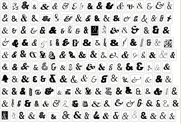
I found over 100k distinct instances of digital letter 'A' from just one day's crawl worth of documents from the web. Some more examples are here
Chances are that the ideas for human-level classifier are out there. They just haven't been implemented and tested in realistic conditions. We need someone with ML/Vision background to come to Google and implement a great character classifier.
You'd have a large impact if your ideas become part of Tesseract. Through books alone, your code will be run on books from 42 libraries. And since Tesseract is open-source, you'd be contributing to the main OCR effort in the open-source community.
You will get a ton of data, resources and smart people around you. It's a very low bureocracy place. You could run Matlab code on 10k cores if you really wanted, and I know someone who has launched 200k core jobs for a personal project. The infrastructure also makes things easier. Google's MapReduce can sort a petabyte of data (10 trillion strings) with 8000 machines in just 30 mins. Some of the work in our team used features coming from distributed deep belief infrastructure.
In order to get an internship position, you must pass general technical screen that I have no control of. If you are interested in more details, you could contact me directly.
Link to apply is here
For example, when I showed the picture below to my Taiwanese coworker he immediately said that these were multiple instance of Chinese "one".

Here are 4 of those images close-up. Classical OCR approaches, have trouble with these characters.

This is a common problem for high-noise domain like camera pictures and digital text rasterized at low resolution. Some results suggest that techniques from Machine Vision can help.
For low-noise domains like Google Books and broken PDF indexing, shortcomings of traditional OCR systems are due to
1) Large number of classes (100k letters in Unicode 6.0)
2) Non-trivial variation within classes
Example of "non-trivial variation"

I found over 100k distinct instances of digital letter 'A' from just one day's crawl worth of documents from the web. Some more examples are here
Chances are that the ideas for human-level classifier are out there. They just haven't been implemented and tested in realistic conditions. We need someone with ML/Vision background to come to Google and implement a great character classifier.
You'd have a large impact if your ideas become part of Tesseract. Through books alone, your code will be run on books from 42 libraries. And since Tesseract is open-source, you'd be contributing to the main OCR effort in the open-source community.
You will get a ton of data, resources and smart people around you. It's a very low bureocracy place. You could run Matlab code on 10k cores if you really wanted, and I know someone who has launched 200k core jobs for a personal project. The infrastructure also makes things easier. Google's MapReduce can sort a petabyte of data (10 trillion strings) with 8000 machines in just 30 mins. Some of the work in our team used features coming from distributed deep belief infrastructure.
In order to get an internship position, you must pass general technical screen that I have no control of. If you are interested in more details, you could contact me directly.
Link to apply is here
Saturday, September 24, 2011
Don't test for exact equality of floating point numbers
A discussion came up on Guido von Rossum's Google Plus post. It comes down to the fact that 2.1 is not exactly represented as a floating point number. Internally it's 2.0999999999999996, and this causes unexpected behavior.
These kinds of issues often come up. The confusion is caused by treating floating point numbers as exact numbers, and expecting calculations with them to produce results meaningful down to the last bit.
It is not in any way "solvable", at least not by means accessible to us (which in some sense defines it as "not a problem"). Depends too much on alignment-handling vagaries of MKL libraries, ordering of operations in BLAS, and usage, or not, of extended precision registers. See also IEEE 754: a careful reading may shed light on how different results for the same computation can arise in compliant hardware/software, even on the same machine
In addition to ambiguity in IEEE 754, which gives slight differences between different floating point libraries, there's an issue of the same library giving slightly different results on reruns with same inputs and and same machine, because of run-time optimization by the processor
The solution that Wolfram Inc came up with is to treat the last 7 bits of IEEE doubles as unknown. When testing for equality, those bits are ignored. When printing a number, it chooses representation that gives a nice printout. For instance, Print[2.0999999999999996] will display 2.1
So here's the rule of thumb for IEEE 754 floating point numbers:
When checking for equality of floating point doubles, ignore the last 7 bits of the mantissa.
Thursday, September 08, 2011
notMNIST dataset
I've taken some publicly available fonts and extracted glyphs from them to make a dataset similar to MNIST. There are 10 classes, with letters A-J taken from different fonts.
Here are some examples of letter "A"
 Judging by the examples, one would expect this to be a harder task than MNIST. This seems to be the case -- logistic regression on top of stacked auto-encoder with fine-tuning gets about 89% accuracy whereas same approach gives got 98% on MNIST.
Dataset consists of small hand-cleaned part, about 19k instances, and large uncleaned dataset, 500k instances. Two parts have approximately 0.5% and 6.5% label error rate. I got this by looking through glyphs and counting how often my guess of the letter didn't match it's unicode value in the font file.
Matlab version of the dataset (.mat file) can be accessed as follows:
load('notMNIST_small.mat')
for i=1:5
    figure('Name',num2str(labels(i))),imshow(images(:,:,i)/255)
end
Zipped version is just a set of png images grouped by class. You can turn zipped version of dataset into Matlab version as follows
tar -xzf notMNIST_large.tar.gz
python matlab_convert.py notMNIST_large notMNIST_large.mat
Approaching 0.5% error rate on notMNIST_small would be very impressive. If you run your algorithm on this dataset, please let me know your results.
Tuesday, August 16, 2011
Making self-contained Unix programs with CDE

In the old days you could statically link your program and run it on another Unix station without worrying about dependencies. Unfortunately static linking no longer works, so you need to make sure that your target platform has the right libraries.
For instance, in order to get Matlab compiled code running on a server, you have to copy over libraries and set environment variables as specified in Matlab's guide, followed by some investigative work to take care of dependencies and version conflicts not covered by Mathworks documentation.
Another example is when if you want to create a self-contained Scipy/Python environment that you could just copy over and use without needing to run configure and make.
For both cases Philip Guo's CDE tool comes helpful. It analyzes your program to find dependencies and makes a package with all the dependencies included. Then it runs the program through a kind of lightweight virtualization, intercepting program calls to trick it into thinking it's running in the original environment.
For instance, here's how you could make a self-contained environment for Python and Scipy:
cd /temp

git clone git://github.com/pgbovine/CDE.git

cd CDE

make

cd ..

CDE/cde python -c "from scipy import *; print zeros(15)"

tar -cf package.tar cde-package
This makes a 26 MB file that includes that all files that were read during execution of that command.
Now you can move it to another machine that doesn't have scipy, prepare the environment and try it out as follows
tar -xf package.tar

cd cde-package/cde-root/temp

../../cde-exec python -c "from scipy import *; print ones(15)"
This will work even if machine doesn't have Python installed, or has the wrong version of shared libraries installed, because cde-exec is reproducing the environment of the original machine. It works for anything that doesn't need files other than the ones accessed during package creation.
For instance, you could start an interactive Python session and run some SciPy examples like this
cde cde-package/cde-root

../cde-exec python

>>> from scipy import *

>>> ....
You could give your containerized program access to host system by creating symlink to the outside in cde-root
Wednesday, July 13, 2011
Google+ ML people
Google+ seems to have a fair number of Machine Learning people, I was able to track down 50 people I've met at conferences by starting at Andrew McCallum's circles. If you add me on Google Circles I'll assume you came from this blog and add you to my "Machine Learning" circle
Saturday, June 25, 2011
Embracing non-determinism

Computers are supposed to be deterministic. This is often the case for single processor machines. However, as you scale up, guaranteeing determinism becomes increasingly expensive.
Even on single processor machines you are facing non-determinism on semi-regular basis. Here are some examples
- Bugs + poor OS memory control that allows programs to read uninitialized memory. A recent example for me was when I used FontForge to process a large set of files, and had it crash on a different set every time I ran it.
- /dev/random gives "truly random" numbers, however, even if the program uses regular rand() seeded by time, it's essentially non-deterministic since so many factors affect the time of seed()
- Floating point operations on modern architecture are non-deterministic because of run-time optimization -- depending on the pattern of memory allocation, processor will rearrange the order of your arithmetic operations, producing slightly different results on reruns
- Soft-errors in circuits due to radiation, about one error per day, according to stats here
- Some CPU units are bad and produce incorrect results. I don't know exact stats on this, but the guy who did the Petasort experiment told me that it was one of the issues they had to deal with.
Those modes of failure may be rare on one computer, but once you scale your computation up to many cores, it becomes a fact of life.
In a distributed application like sorting a petabyte of data, you should expect about 1 hardrive failure, 100 irrecoverable disk read errors, and a couple of undetected memory errors if you use error correcting RAM (more if you use regular RAM).
You can make your computation deterministic by adding checksums at each stage and recomputing the parts that fail. However, this is expensive, and becomes disporportionately more expensive as you scale up. When the Czajkowski et al sorted 100 trillion records deterministically, most of the time was spent on error recovery.
I've been running an aggregation that is modest in comparison, going over over about 100 TB of data and getting slightly different results each time. Theoretically I could add recovery stages that get rid of non-determinism, but at a cost that is not justified in my case.
Large scale analysis systems like Dremel are configured to produce approximate results by default, otherwise, the long tail of packet arrival times means that you'll spent most of the time waiting for a few "stragglers"
Given the increasing cost of determinism it makes sense to think of it in terms of cost-benefit analysis and trade off the benefit of reproducible results against the cost of 100% error recovery.
A related idea come up in Vikash Mansinghka presentation at NIPS 2010 workshop on monte carlo methods: Real world decision problems can be formulated as inference and solved with MCMC sampling, so it doesn't make sense to spend so much effort ensuring determinism only to destroy it with /dev/random -- you could achieve greater efficiency by using analogue circuits to start with. His company, Navia, is working in this direction.
There's some more discussion on determinism on Daniel Lemire's blog
Wednesday, June 22, 2011
Machine Learning opportunities at Google
Google is hiring and there are lots of opportunities to do Machine Learning-related work here. Kevin Murphy is applying Bayesian methods to video recommendation, Andrew Ng is working on a neural network that can run on millions of cores, and that's just the tip of the iceberg that I've discovered working here for last 3 months.
There is machine learning work in both "researcher" and "engineer" positions, and the focus on applied research makes the distinction somewhat blurry.
There is machine learning work in both "researcher" and "engineer" positions, and the focus on applied research makes the distinction somewhat blurry.
Saturday, April 30, 2011
Neural Networks making a come-back?
Five years ago I ran some queries on Google Scholar to see trends on the number of papers that mention particular phrase. The number of hits for each year was divided by the number of hits for "machine learning". Back then it looked like NN's started gaining in popularity with invention of back-propagation in 1980's, peaked in 1993 and went downhill from there.
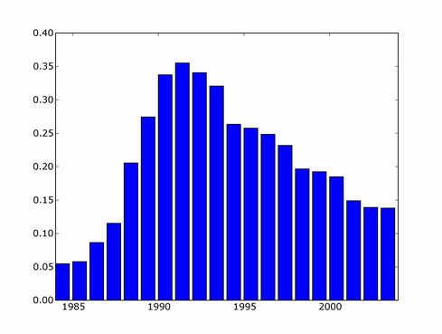
Since then, there's been several major NN developments, involving deep learning and probabilistically founded versions so I decided to update the trend. I couldn't find a copy of scholar scraper script anymore, luckily Konstantin Tretjakov has maintained a working version and reran the query for me.
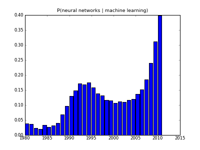
It looks like downward trend in 2000's was misleading because not all papers from that period have made it into index yet, and the actual recent trend is exponential growth!
One example of this "third wave" of Neural Network research is unsupervised feature learning. Here's what you get if you train a sparse auto-encoder on some natural scene images
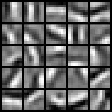
What you get is pretty much a set of Gabor filters, but the cool thing is that you get them from your neural network rather than image processing expert

Since then, there's been several major NN developments, involving deep learning and probabilistically founded versions so I decided to update the trend. I couldn't find a copy of scholar scraper script anymore, luckily Konstantin Tretjakov has maintained a working version and reran the query for me.

It looks like downward trend in 2000's was misleading because not all papers from that period have made it into index yet, and the actual recent trend is exponential growth!
One example of this "third wave" of Neural Network research is unsupervised feature learning. Here's what you get if you train a sparse auto-encoder on some natural scene images

What you get is pretty much a set of Gabor filters, but the cool thing is that you get them from your neural network rather than image processing expert
Friday, April 29, 2011
Another ML blog
I just noticed that Justin Domke has a blog --
He's one of the strongest researchers in the field of graphical models. I first came across his dissertation when looking for a way to improve loopy-Belief Propagation based training. His thesis gives one such idea -- instead of maximizing the fit of an intractable model, and using BP as intermediate step, maximize the fit of BP marginals directly. This makes sense since approximate (BP-based) marginals are what you ultimately use.
If you run BP for k steps, then likelihood of the BP-approximated model is tractable to minimize -- calculation of gradient is very similar to k steps of loopy BP. I derived formulas for gradient of "BP-approximated likelihood" in equations 17-21 in this note. It looks a bit complicated in my notation, but derivation is basically an application of chain rule to BP-marginal, which is a composition of k-steps of BP update formula.
Sunday, March 13, 2011
Going to Google
I've accepted an offer from Google and will be joining their Tesseract team next week.
I first got interested in OCR when I faced a project at my previous job involving OCR of outdoor scenes and found it to be a very complex task, yet highly rewarding because it's easy to make incremental progress and see your learners working.
Current state-of-the-art OCR tools are not at human level of reading, partially because humans are able to take context into account. For instance, sentence below is unreadable if you don't assume English language.

Also, I'm excited to work on an open-source project. I'd like to live in a world where the best technologies are open-source and free to everyone.
I first got interested in OCR when I faced a project at my previous job involving OCR of outdoor scenes and found it to be a very complex task, yet highly rewarding because it's easy to make incremental progress and see your learners working.
Current state-of-the-art OCR tools are not at human level of reading, partially because humans are able to take context into account. For instance, sentence below is unreadable if you don't assume English language.

Also, I'm excited to work on an open-source project. I'd like to live in a world where the best technologies are open-source and free to everyone.
Saturday, March 05, 2011
Linear Programming for Maximum Independent Set
Maximum independent set, or "maximum stable" set is one of classical NP-complete problems described in Richard Karp's 1972 paper "Reducibility Among Combinatorial Problems". Other NP-complete problems often have a simple reduction to it, for instance, p.3 of Tony Jebara's "MAP Estimation, Message Passing, and Perfect Graphs" shows how MAP inference in an arbitrary MRF reduces to Maximum Weight Independent Set.
The problem asks to find the largest set of vertices in a graph, such that no two vertices are adjacent.
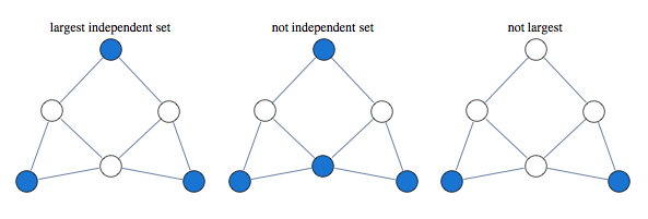
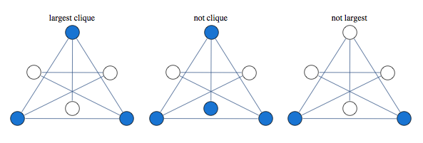
Finding largest independent set is equivalent to finding largest clique in graph's complement
A classical approach to solving this kind of problem is based on linear relaxation.
Take a variable for every vertex of the graph, let it be 1 if vertex is occupied and 0 if it is not occupied. We encode independence constraint by requiring that adjacent variables add up to 1. So we can consider the following graph and corresponding integer programming formulation:

$$\max x_1 + x_2 + x_3 + x_4 $$
such that
$$
\begin{array}{c}
x_1+x_2 \le 1 \\\\
x_2+x_3 \le 1 \\\\
x_3+x_4 \le 1 \\\\
x_4+x_1 \le 1 \\\\
x_i\ge 0 \ \ \forall i \\\\
x_i \in \text{Integers}\ \forall i
\end{array}
$$
Solving this integer linear integer program is equivalent to the original problem of maximum independent set, with 1 value indicating that node is in the set. To get a tractable LP programme we drop the last constraint.
If we solve LP without integer constraints and get integer valued result, the result is guaranteed to be correct. In this case we say that LP is tight, or LP is integral.
Curiously, solution of this kind of LP is guaranteed to take only values 0,1 and $\frac{1}{2}$. This is known as "half-integrality". Integer valued variables are guaranteed to be correct, and we need to use some other method to determine assignments to half-integer variables.
For instance below is a graph for which first three variables get 1/2 in the solution of the LP, while the rest of the vertices get integral values which are guaranteed to be correct

Here's what this LP approach gives us for a sampling of graphs

A natural question to ask is when this approach works. Its guaranteed to work for bipartite graphs, but it also seems to work for many non-bipartite graphs. None of the graphs above are bipartite.
Since independent set only allows one vertex per clique, we can improve our LP by saying that sum of variables over each clique has to below 1.
Consider the following graph that our original LP has a problem with:

Instead of having edge constraints, we formulate our LP with clique constraints as follows:
$$x_1+x_2+x_3\le 1$$
$$x_3+x_4+x_5\le 1$$
With these constraints, LP solver is able to find the integral solution

In this formulation, solution of LP is no longer half-integral. For the graph below we get a mixture of 1/3 and 2/3 in the solution.

Optimum of this LP is known as the "fractional chromatic number" and it is an upper bound both on the largest clique size and the largest independent set size. For the graph above, largest clique and independent set have sizes 9/3 and 12/3, whereas fractional chromatic number is 14/3.
This relaxation is tighter than previous, here are some graphs that previous LP relaxation had a problem with.

This LP is guaranteed to work for perfect graphs which is a larger class of graphs than bipartite graphs. Out of 853 connected graphs over 7 vertices, 44 are bipartite while 724 are perfect.
You can improve this LP further by adding more constraints. A form of LP constraints that generalizes previous two approaches is
$$\sum_{i\in C} x_i\le \alpha(C)$$
Where $C$ is some subgraph and $\alpha(C)$ is its independence number.
You extend previous relaxation by considering subgraphs other than cliques.
Lovasz describes the following constraint classes (p.13 of "Semidefinite programs and combinatorial optimization")
1. Odd hole constraints
2. Odd anti-hole constraints
3. Alpha-critical graph constraints.
Note that adding constraints for all maximal cliques can produce a LP with exponential number of constraints.
Notebook
Packages
The problem asks to find the largest set of vertices in a graph, such that no two vertices are adjacent.

Finding largest independent set is equivalent to finding largest clique in graph's complement

A classical approach to solving this kind of problem is based on linear relaxation.
Take a variable for every vertex of the graph, let it be 1 if vertex is occupied and 0 if it is not occupied. We encode independence constraint by requiring that adjacent variables add up to 1. So we can consider the following graph and corresponding integer programming formulation:

$$\max x_1 + x_2 + x_3 + x_4 $$
such that
$$
\begin{array}{c}
x_1+x_2 \le 1 \\\\
x_2+x_3 \le 1 \\\\
x_3+x_4 \le 1 \\\\
x_4+x_1 \le 1 \\\\
x_i\ge 0 \ \ \forall i \\\\
x_i \in \text{Integers}\ \forall i
\end{array}
$$
Solving this integer linear integer program is equivalent to the original problem of maximum independent set, with 1 value indicating that node is in the set. To get a tractable LP programme we drop the last constraint.
If we solve LP without integer constraints and get integer valued result, the result is guaranteed to be correct. In this case we say that LP is tight, or LP is integral.
Curiously, solution of this kind of LP is guaranteed to take only values 0,1 and $\frac{1}{2}$. This is known as "half-integrality". Integer valued variables are guaranteed to be correct, and we need to use some other method to determine assignments to half-integer variables.
For instance below is a graph for which first three variables get 1/2 in the solution of the LP, while the rest of the vertices get integral values which are guaranteed to be correct

Here's what this LP approach gives us for a sampling of graphs

A natural question to ask is when this approach works. Its guaranteed to work for bipartite graphs, but it also seems to work for many non-bipartite graphs. None of the graphs above are bipartite.
Since independent set only allows one vertex per clique, we can improve our LP by saying that sum of variables over each clique has to below 1.
Consider the following graph that our original LP has a problem with:

Instead of having edge constraints, we formulate our LP with clique constraints as follows:
$$x_1+x_2+x_3\le 1$$
$$x_3+x_4+x_5\le 1$$
With these constraints, LP solver is able to find the integral solution

In this formulation, solution of LP is no longer half-integral. For the graph below we get a mixture of 1/3 and 2/3 in the solution.

Optimum of this LP is known as the "fractional chromatic number" and it is an upper bound both on the largest clique size and the largest independent set size. For the graph above, largest clique and independent set have sizes 9/3 and 12/3, whereas fractional chromatic number is 14/3.
This relaxation is tighter than previous, here are some graphs that previous LP relaxation had a problem with.

This LP is guaranteed to work for perfect graphs which is a larger class of graphs than bipartite graphs. Out of 853 connected graphs over 7 vertices, 44 are bipartite while 724 are perfect.
You can improve this LP further by adding more constraints. A form of LP constraints that generalizes previous two approaches is
$$\sum_{i\in C} x_i\le \alpha(C)$$
Where $C$ is some subgraph and $\alpha(C)$ is its independence number.
You extend previous relaxation by considering subgraphs other than cliques.
Lovasz describes the following constraint classes (p.13 of "Semidefinite programs and combinatorial optimization")
1. Odd hole constraints
2. Odd anti-hole constraints
3. Alpha-critical graph constraints.
Note that adding constraints for all maximal cliques can produce a LP with exponential number of constraints.
Notebook
Packages
Thursday, March 03, 2011
Perils of floating point arithmetic
A recent discussion on stackoverflow brought up the issue of results of floating point arithmetic being non-reproducible
A reader asked what one could do to guarantee that result of floating point computation is always the same, and Daniel Lichtblau, a veteran developer at the kernel group of WRI replied that "it is impossible with current hardware and software"
One problem is that IEEE 754 standard is ambiguous, and different implementations of it give slightly different results. See page 250 of What Every Computer Scientist Should Know About Floating Point Arithmetic for specific examples. This means that compiling code on a different system can produce slightly different results.
Another issue is that even when you run the same computation on the same system, results can be slightly different on reruns. This has to do with how low-level optimization is scheduled.
This means that if you want your results to be reproducible, you should avoid things like testing floating point numbers for equality. John D Cook gives some more advice in Five Tips for Floating Point Programming
Monday, February 21, 2011
How to patent an algorithm in the US
Today I got Google Alert today on the following pending patent -- Belief Propagation for Generalized Matching. I like to stay up on Belief Propagation literature, so I took a closer look. The PDF linked gives a fairly detailed explanation of belief propagation for solving matching problems, including pseudocode which is very detailed, looking like an excerpt of a C program. Appendix A seems to be an expanded version of a paper which appeared in NIPS 2008 workshop
A pecularity of the US patent system is that patents on algorithms are not allowed, yet algorithms are frequently patented. A few years ago when I blogged on the issue of patents in Machine Learning, I didn't know the specifics, but now, having gone through the process, I know a bit more.
When filing an algorithm patent, patent lawyer will tell you to remove every instance of the word "algorithm" and replace it with some other word. This seems to be necessary for getting the patent through.
So, in the patent above, belief propagation algorithm is referred to as "belief propagation system". In the whole application, word "system" occurs 114 times, whereas "algorithm" occurs 1 time, in reference to a competing approach.
Another thing the patent lawyer will probably ask for is lots and lots of diagrams. I'm guessing that diagrams serve as further evidence that your algorithm is a "system" and not merely an algorithm. There are only so many useful diagrams you can have, so at some point you may find yourself pulling diagrams from thin ar and thinking "why am I doing this?" (but then remembering that it's because of the bonus). In the industry, a common figure seems to be $5000 for a patent that goes through. If a company doesn't have bonus structure, they may use other means to pressure employees into patent process. (note, patent above was filed through a university)
As a result, these kinds of patents end up with vacuous diagrams.
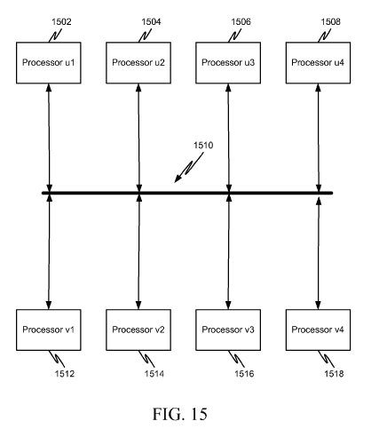
For instance, In the patent above, there are 17 figures, and a few of them don't seem to convey any useful information. The one below is illustrating the "plurality of belief propagation processors connected to a bus"
And this one is one is to illustrate belief propagation processors connected to a network
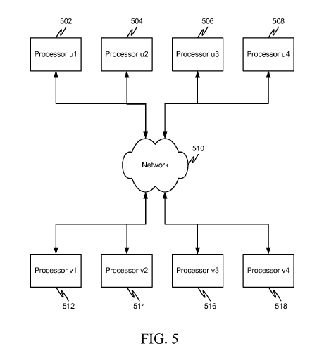
Finally when I saw the following diagram, I first thought it was there to illustrate BP update formula, which involves adding and multiplying numbers
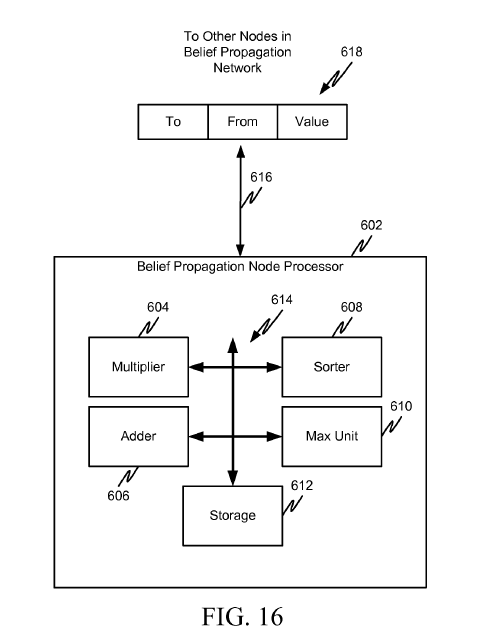
But it's not even tenuously connected to the rest of the patent. 604 is supposed to be "computer readable media", 606 is a "link that couples media to the network", 608 is the "network" for aforementioned "link" and "media". 616 and 618 are not referenced.
This doesn't actually matter because nobody really reads the patent anyway. The most important part of getting the patent through is having a patent lawyer on the case who can frame it in the right format and handle communication with the patent office. The process for regular (non-expedited) patents can take five years and the total cost can exceed $50,000.
As to why an organization would spend so much time and money on a patent that might not even be enforceable by virtue of being an algorithm patent -- patents have intrinsic value. Once patent clears the patent office, a patent is an asset which can be sold or traded and as a result increases company worth. You can sell rights to pending patents before they are granted which makes the actual content of the patent even less important
A pecularity of the US patent system is that patents on algorithms are not allowed, yet algorithms are frequently patented. A few years ago when I blogged on the issue of patents in Machine Learning, I didn't know the specifics, but now, having gone through the process, I know a bit more.
When filing an algorithm patent, patent lawyer will tell you to remove every instance of the word "algorithm" and replace it with some other word. This seems to be necessary for getting the patent through.
So, in the patent above, belief propagation algorithm is referred to as "belief propagation system". In the whole application, word "system" occurs 114 times, whereas "algorithm" occurs 1 time, in reference to a competing approach.
Another thing the patent lawyer will probably ask for is lots and lots of diagrams. I'm guessing that diagrams serve as further evidence that your algorithm is a "system" and not merely an algorithm. There are only so many useful diagrams you can have, so at some point you may find yourself pulling diagrams from thin ar and thinking "why am I doing this?" (but then remembering that it's because of the bonus). In the industry, a common figure seems to be $5000 for a patent that goes through. If a company doesn't have bonus structure, they may use other means to pressure employees into patent process. (note, patent above was filed through a university)
As a result, these kinds of patents end up with vacuous diagrams.
For instance, In the patent above, there are 17 figures, and a few of them don't seem to convey any useful information. The one below is illustrating the "plurality of belief propagation processors connected to a bus"

And this one is one is to illustrate belief propagation processors connected to a network

Finally when I saw the following diagram, I first thought it was there to illustrate BP update formula, which involves adding and multiplying numbers

But it's not even tenuously connected to the rest of the patent. 604 is supposed to be "computer readable media", 606 is a "link that couples media to the network", 608 is the "network" for aforementioned "link" and "media". 616 and 618 are not referenced.
This doesn't actually matter because nobody really reads the patent anyway. The most important part of getting the patent through is having a patent lawyer on the case who can frame it in the right format and handle communication with the patent office. The process for regular (non-expedited) patents can take five years and the total cost can exceed $50,000.
As to why an organization would spend so much time and money on a patent that might not even be enforceable by virtue of being an algorithm patent -- patents have intrinsic value. Once patent clears the patent office, a patent is an asset which can be sold or traded and as a result increases company worth. You can sell rights to pending patents before they are granted which makes the actual content of the patent even less important
Sunday, February 20, 2011
Generalized Distributive Law
With regular distributive law you can do things like
$$\sum_{x_1,x_2,x_3} \exp(x_1 + x_2 + x_3)=\sum_{x_1} \exp x_1 \sum_{x_2} \exp x_2 \sum_{x_3} \exp x_3$$
This breaks the original large sum into 3 small sums which can be computed independently.
A more realistic scenario requires factorization into overlapping parts. For instance take the following
$$\sum_{x1,x2,x3,x_4,x_5} \exp(x_1 x_2 + x_2 x_3 + x_3 x_4+x_4 x_5)$$
You can't use directly apply distributive law here. Naive evaluation of the sum is exponential in the number of variables, however this problem can be solved in time linear in the number of variables.
Consider the following factorization
$$\sum_{x1,x2} \exp x_1 x_2 \left( \sum_{x_3} \exp x_2 x_3 \left( \sum_{x_4} \exp x_3 x_4 \left( \sum_{x_5} \exp x_4 x_5 \right) \right) \right) $$
Now note that when computing inner sums, naive approach results in same sum being recomputed many times. Save those shared pieces and you get an algorithm that's quadratic in number of variable values and linear in number of variables
Viterbi and Forward-Backward are specific names of this kind of dynamic programming for chain structured sums as above.
To consider tree-structured sum, take a problem of counting independent sets in a tree-structured graph. In this case we can use the following factorization


This is the first step of the recursion and you can repeat it until your pieces have tractable size.
Now for a general case of non-tree-structured graph, consider the sum below
$$\sum_{x1,x2,x3,x_4,x_5} \exp( x_1 x_2 + x_2 x_3 + x_3 x_4+x_4 x_5 + x_5 x_1 )$$
Here, variables form a loop, so regular tree recursion like Viterbi does not apply. However, this sum can be found efficiently, linear in the number of variables, and cubically in the number of variable values. I have more in depth explanation of decomposing problems like above in an answer on cstheory site but the basic idea is similar to the approach with independent sets -- fix some variables and recurse on subparts.
This kind of general factorization has been re-invented many times and is known as Generalized Distributive Law, tree-decomposition, junction tree, clique tree, partial k-tree, and probably a few other names.
Notebook
$$\sum_{x_1,x_2,x_3} \exp(x_1 + x_2 + x_3)=\sum_{x_1} \exp x_1 \sum_{x_2} \exp x_2 \sum_{x_3} \exp x_3$$
This breaks the original large sum into 3 small sums which can be computed independently.
A more realistic scenario requires factorization into overlapping parts. For instance take the following
$$\sum_{x1,x2,x3,x_4,x_5} \exp(x_1 x_2 + x_2 x_3 + x_3 x_4+x_4 x_5)$$
You can't use directly apply distributive law here. Naive evaluation of the sum is exponential in the number of variables, however this problem can be solved in time linear in the number of variables.
Consider the following factorization
$$\sum_{x1,x2} \exp x_1 x_2 \left( \sum_{x_3} \exp x_2 x_3 \left( \sum_{x_4} \exp x_3 x_4 \left( \sum_{x_5} \exp x_4 x_5 \right) \right) \right) $$
Now note that when computing inner sums, naive approach results in same sum being recomputed many times. Save those shared pieces and you get an algorithm that's quadratic in number of variable values and linear in number of variables
Viterbi and Forward-Backward are specific names of this kind of dynamic programming for chain structured sums as above.
To consider tree-structured sum, take a problem of counting independent sets in a tree-structured graph. In this case we can use the following factorization


This is the first step of the recursion and you can repeat it until your pieces have tractable size.
Now for a general case of non-tree-structured graph, consider the sum below
$$\sum_{x1,x2,x3,x_4,x_5} \exp( x_1 x_2 + x_2 x_3 + x_3 x_4+x_4 x_5 + x_5 x_1 )$$
Here, variables form a loop, so regular tree recursion like Viterbi does not apply. However, this sum can be found efficiently, linear in the number of variables, and cubically in the number of variable values. I have more in depth explanation of decomposing problems like above in an answer on cstheory site but the basic idea is similar to the approach with independent sets -- fix some variables and recurse on subparts.
This kind of general factorization has been re-invented many times and is known as Generalized Distributive Law, tree-decomposition, junction tree, clique tree, partial k-tree, and probably a few other names.
Notebook
Tuesday, February 15, 2011
Cluster decomposition and variational counting
Suppose we want to count the number of independent sets in a graph below.

There are 9 independent sets.

Because the graphs are disjoint we could simplify the task by counting graphs in each connected component separately and multiplying the result

Variational approach is one way of extending this decomposition idea to connected graphs.
Consider the problem of counting independent sets in the following graph.

There are 7 independent sets. Let $x_i=1$ indicate that node $i$ is occupied, and $P(x_1,x_2,x_3,x_4)$ be a uniform distribution over independent sets, meaning it is either 1/7 or 0 depending whether $x_1,x_2,x_3,x_4$ forms an independent set
Entropy of uniform distribution over $n$ independent sets distribution is $H=-\log(1/n)$, hence $n=\exp H$, so to find the number of independent sets just find the entropy of distribution $P$ and exponentiate it.
We can represent P as follows
$$P(x_1,x_2,x_3,x_4)=\frac{P_a(x_1,x_2,x_3)P_b(x_1,x_3,x_4)}{P_c(x_1,x_3)}$$
Entropy of P similarly factorizes
$$H=H_a + H_b - H_c$$
Once you have $P_A$, $P_B$ and $P_C$ representing our local distributions of our factorization, we can forget the original graph and compute the number of independent sets from entropies of these factors
To find factorization of $P$ into $P_a,P_b$, and $P_c$ minimize the following objective
$$KL(\frac{P_a P_b}{P_c},P)$$
This is KL-divergence between our factorized representation and original representation. Message passing schemes like cluster belief propagation can be derived as one approach of solving this minimization problem. In this case, cluster belief propagation takes 2 iterations to find the minimum of this objective. Note that the particular form of distance is important. We could reverse the order and instead minimize $KL(P,P_a P_b/P_c)$ and while this makes sense from approximation stand-point, minimizing reversed form of KL-divergence is generally intractable.
This decomposition is sufficiently rich that we can model P exactly using proper choice of $P_a,P_b$ and $P_c$, so the minimum of our objective is 0, and our entropy decomposition is exact.
Now, the number of independent sets using decomposition above factorizes as
$$n=\exp H=\frac{\exp H_a \exp H_b}{\exp H_c} = \frac{\left(\frac{7}{2^{4/7}}\right)^2}{\frac{7}{2\ 2^{1/7}}} = \frac{4.75 \times 4.75}{3.17}=7$$
Our decomposition can be schematically represented as the following cluster graph

We have two regions and we can think of our decomposition as counting number of independent sets in each region, then dividing by number of independent sets in the vertex set shared by pair of connected regions. Note that region A gets "4.75 independent sets" so this is not as intuitive as decomposition into connected components
Here's another example of graph and its decomposition.


Using 123 to refer to $P(x_1,x_2,x_3)$ the formula representing this decomposition is as follows
$$\frac{124\times 236\times 2456 \times 4568 \times 478\times 489}{24\times 26 \times 456 \times 48 \times 68}$$
There are 63 independent sets in this graph, and using decomposition above the count decomposes as follows:
$$63=\frac{\left(\frac{21\ 3^{5/7}}{2\ 2^{19/21} 5^{25/63}}\right)^2 \left(\frac{3\ 21^{1/3}}{2^{16/21} 5^{5/63}}\right)^4}{\frac{21\ 3^{3/7}}{2\ 2^{1/7} 5^{50/63}} \left(\frac{3\ 21^{1/3}}{2\ 2^{3/7} 5^{5/63}}\right)^4}$$
Finding efficient decomposition that models distribution exactly requires that graph has small tree-width. This is not the case for many graphs, such as large square grids, but we can apply the same procedure to get cheap inexact decomposition.
Consider the following inexact decomposition of our 3x3 grid

Corresponding decomposition has 4 clusters and 4 separators, and the following factorization formula
$$\frac{1245\times 2356 \times 4578 \times 5689}{25\times 45 \times 56 \times 58}$$
We can use minimization objective as before to find the parameters of this factorization. Since original distribution can not be exactly represented in this factorization, result will be approximate, unlike previous two example.
Using message-passing to solve the variational problem takes about 20 iterations to converge, to an estimate of 46.97 independent sets

To try various decompositions yourself, unzip the archive and look at usage examples in indBethe3-test.nb
Notebooks

There are 9 independent sets.

Because the graphs are disjoint we could simplify the task by counting graphs in each connected component separately and multiplying the result

Variational approach is one way of extending this decomposition idea to connected graphs.
Consider the problem of counting independent sets in the following graph.

There are 7 independent sets. Let $x_i=1$ indicate that node $i$ is occupied, and $P(x_1,x_2,x_3,x_4)$ be a uniform distribution over independent sets, meaning it is either 1/7 or 0 depending whether $x_1,x_2,x_3,x_4$ forms an independent set
Entropy of uniform distribution over $n$ independent sets distribution is $H=-\log(1/n)$, hence $n=\exp H$, so to find the number of independent sets just find the entropy of distribution $P$ and exponentiate it.
We can represent P as follows
$$P(x_1,x_2,x_3,x_4)=\frac{P_a(x_1,x_2,x_3)P_b(x_1,x_3,x_4)}{P_c(x_1,x_3)}$$
Entropy of P similarly factorizes
$$H=H_a + H_b - H_c$$
Once you have $P_A$, $P_B$ and $P_C$ representing our local distributions of our factorization, we can forget the original graph and compute the number of independent sets from entropies of these factors
To find factorization of $P$ into $P_a,P_b$, and $P_c$ minimize the following objective
$$KL(\frac{P_a P_b}{P_c},P)$$
This is KL-divergence between our factorized representation and original representation. Message passing schemes like cluster belief propagation can be derived as one approach of solving this minimization problem. In this case, cluster belief propagation takes 2 iterations to find the minimum of this objective. Note that the particular form of distance is important. We could reverse the order and instead minimize $KL(P,P_a P_b/P_c)$ and while this makes sense from approximation stand-point, minimizing reversed form of KL-divergence is generally intractable.
This decomposition is sufficiently rich that we can model P exactly using proper choice of $P_a,P_b$ and $P_c$, so the minimum of our objective is 0, and our entropy decomposition is exact.
Now, the number of independent sets using decomposition above factorizes as
$$n=\exp H=\frac{\exp H_a \exp H_b}{\exp H_c} = \frac{\left(\frac{7}{2^{4/7}}\right)^2}{\frac{7}{2\ 2^{1/7}}} = \frac{4.75 \times 4.75}{3.17}=7$$
Our decomposition can be schematically represented as the following cluster graph

We have two regions and we can think of our decomposition as counting number of independent sets in each region, then dividing by number of independent sets in the vertex set shared by pair of connected regions. Note that region A gets "4.75 independent sets" so this is not as intuitive as decomposition into connected components
Here's another example of graph and its decomposition.


Using 123 to refer to $P(x_1,x_2,x_3)$ the formula representing this decomposition is as follows
$$\frac{124\times 236\times 2456 \times 4568 \times 478\times 489}{24\times 26 \times 456 \times 48 \times 68}$$
There are 63 independent sets in this graph, and using decomposition above the count decomposes as follows:
$$63=\frac{\left(\frac{21\ 3^{5/7}}{2\ 2^{19/21} 5^{25/63}}\right)^2 \left(\frac{3\ 21^{1/3}}{2^{16/21} 5^{5/63}}\right)^4}{\frac{21\ 3^{3/7}}{2\ 2^{1/7} 5^{50/63}} \left(\frac{3\ 21^{1/3}}{2\ 2^{3/7} 5^{5/63}}\right)^4}$$
Finding efficient decomposition that models distribution exactly requires that graph has small tree-width. This is not the case for many graphs, such as large square grids, but we can apply the same procedure to get cheap inexact decomposition.
Consider the following inexact decomposition of our 3x3 grid

Corresponding decomposition has 4 clusters and 4 separators, and the following factorization formula
$$\frac{1245\times 2356 \times 4578 \times 5689}{25\times 45 \times 56 \times 58}$$
We can use minimization objective as before to find the parameters of this factorization. Since original distribution can not be exactly represented in this factorization, result will be approximate, unlike previous two example.
Using message-passing to solve the variational problem takes about 20 iterations to converge, to an estimate of 46.97 independent sets

To try various decompositions yourself, unzip the archive and look at usage examples in indBethe3-test.nb
Notebooks
Wednesday, February 09, 2011
Junction trees in numerical analysis
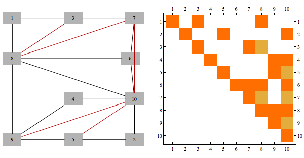
There's a neat connection between Cholesky factorization and graph triangulations -- graph corresponding to Cholesky factorization of a sparse matrix is precisely the triangulation of the sparse matrix (when viewed as a graph) using canonical elimination ordering.
Here's an example of a matrix (corresponding to the graph with black edges only), and its Cholesky factorization. We triangulate the graph by any pairs of neighbors of v which have higher index than v, for every v. Extra edges added in this way correspond to extra non-zero entries in Cholesky decomposition of the original matrix. Different color edges/matrix entries correspond to non-zero entries in Cholesky factorization not present in original matrix
Furthermore, junction tree we get using min-fill heuristic of a graph is same structure as what is used to perform Cholesky factorization using parallel multi-frontal method
Here's a chordal matrix in perfect order and its Cholesky factorization
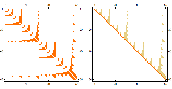
The fact that Cholesky factorization has the same sparsity structure as the original matrix confirms that its a chordal matrix in perfect elimination order
Here's the graph representation of the matrix
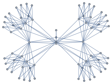
Junction tree decomposition of this graph reveals the following clique structure
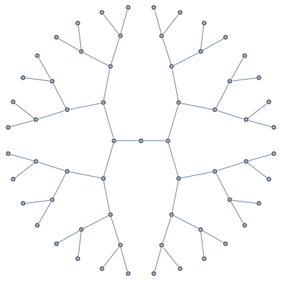
High branching structure of decomposition means that Cholesky factorization can be highly parallelized, in particular, the very last step of Cholesky decomposition of this matrix in minfill order consists of 32 independent tasks that can be done in parallel.
I packaged together some Mathematica code for these kinds of tasks
Here's an example of a matrix (corresponding to the graph with black edges only), and its Cholesky factorization. We triangulate the graph by any pairs of neighbors of v which have higher index than v, for every v. Extra edges added in this way correspond to extra non-zero entries in Cholesky decomposition of the original matrix. Different color edges/matrix entries correspond to non-zero entries in Cholesky factorization not present in original matrix

Furthermore, junction tree we get using min-fill heuristic of a graph is same structure as what is used to perform Cholesky factorization using parallel multi-frontal method
Here's a chordal matrix in perfect order and its Cholesky factorization

The fact that Cholesky factorization has the same sparsity structure as the original matrix confirms that its a chordal matrix in perfect elimination order
Here's the graph representation of the matrix

Junction tree decomposition of this graph reveals the following clique structure

High branching structure of decomposition means that Cholesky factorization can be highly parallelized, in particular, the very last step of Cholesky decomposition of this matrix in minfill order consists of 32 independent tasks that can be done in parallel.
I packaged together some Mathematica code for these kinds of tasks
Friday, January 21, 2011
Building Junction Trees
Here's a 367 vertex Apollonian Network and its Junction Tree (aka Tree Decomposition)
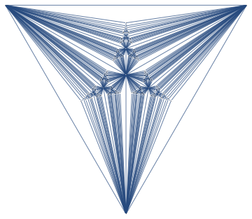
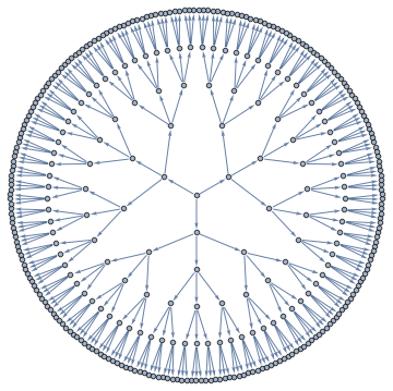
A Junction Tree provides an efficient data structure to do exact probabilistic inference. In the context of traditional graph algorithms, it is known as the "Tree Decomposition". The amount of structure apparent from the junction tree shows that problems structured as Apollonian Networks have very low computational complexity.
The same junction tree structure can also be used to efficiently compute chromatic polynomials, find cliques, count self-avoiding walks, and the reason for this universality is that it essentially captures separation structure of the graph -- it is a representation of a complete set of vertex separators. In the Junction Tree above you can see 121 non-leaf nodes that separate the graph into 3 parts. Each node corresponds to a set of 4 vertices. There are also 363 edges, each corresponds to a set of 3 vertices that separates the graph into 2 parts. The fact that the graph can be recursively partitioned using small separators implies an efficient recursion scheme for problems on this graph.
I put together a Mathematica package to build Junction Trees like above using MinFill, MinCut and a few other heuristics. Some experimenting showed MinFill with Vertex Eccentricity for choosing between vertices with equal fill to work the best for general graphs, whereas MinCut worked the best for planar graphs.
Friday, January 14, 2011
P vs. NP page
Here's a page linking 65 attempts of resolving P vs NP problem. A couple of papers were published in peer-reviewed journals or conferences, while most are "arxiv" published. Some statistics:
- 35 prove P=NP
- 28 prove P!=NP
- 2 prove it can go either way (undecidable)
Saturday, January 08, 2011
towards Problem Compilers
First programmers wrote in machine code and assemblers simplified this task significantly by letting them give algorithms at a higher level. I still find stacks of punch cards like below in my St.Petersburg home
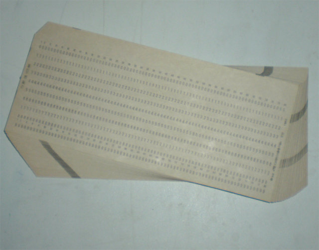
Wouldn't it be great if we could extend this idea further and have the computer compile the problem into machine code?
Actually, we already have such tools restricted to various versions of "problem language". For instance if you express your problem in terms of integer optimization, you can use integer programming tools.
Another language is the language of "graphical models". In the most general formulation, you specify meaning of operations + and *, that obey distributive law, set of x variables, set of functions f, and ask computer to find the following
$$\bigoplus_{x_1,x_2,\ldots} \bigotimes_f f(x)$$
This formulation has a natural "interactions graph" associated with it, and a computer can find an algorithm to solve this problem using tree decomposition if interactions between f functions are not too complex
However, this is still suboptimal because the algorithm designer needs to pick variables x and functions f, and this choice is fairly important. For instance, for minimum weight Steiner Tree, "natural" variables of the problem don't give a good factorization, and you need a smart designer to figure out a good reparameterization of the problem, like here.
As it stands right now, if a designer gives a good parameterization of the problem, a computer can solve it. Can we train a computer to find a parameterization?
I don't know the answer, but one potential approach to finding parameterizations is described in A new look at Generalized Distributive Law. They formulate the problem of optimal decomposition as that of search at the level of individual instantiations of x, so theoretically, this approach can discover optimal parameterization of the problem.
Sunday, January 02, 2011
Interactive Tree Decomposition
Here's a tool (in Mathematica) to help visualize the process of constructing a Junction Tree. wrong link fixed
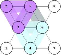
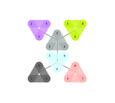
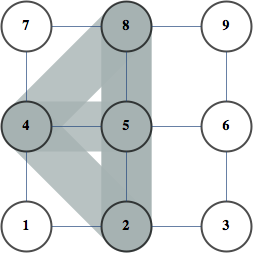
Clicking on vertices corresponds to vertex elimination and each click creates a new bag. After all vertices are eliminated, junction tree is created by removing redundant bags and taking the maximum spanning tree with size of the separators defining the weight of each edge as the junction tree.
If you try it on small examples, you can get some intuition of how outperform the greedy approach -- basically you want to find small separators of the graph, and at the same time you want those separators to have a lot of vertices in common


 |  |

 |  |
Subscribe to:
Comments (Atom)


