Russian CAPTCHA

Here's an innovative CAPTCHA I came across when trying to register for a forum at http://lib.mipt.ru/?spage=reg_user

You have to enter resistance between A and B in the diagram below. Can you do it?

Sampling doubly stochastic matrices

Stochastic matrices are easy to get -- just normalize the rows. Doubly stochastic matrices require more work -- simply normalizing columns/rows will not converge may take few dozen iterations to converge. One approach that works is to do constrained optimization, finding closest (in least squared sense) doubly stochastic matrix to given matrix. Another approach is to start with a permutation matrix and follow a Markov chain that modifies 4 elements randomly at each step in a way that keeps the matrix doubly stochastic. Here is the implementation of these two methods in Mathematica (notebook in the same directory)

http://www.yaroslavvb.com/research/qr/doubly-stochastic/doubly-stochastic.html

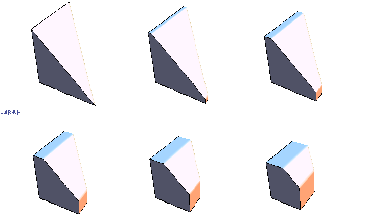
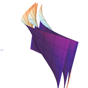
As Jeremy pointed out, Birkhoff's theorem provides necessary and sufficient conditions for a matrix to be doubly stochastic -- it must be a convex combination of permutation matrices. It seems hard to sample from the set of valid convex combinations though. For instance, here's a set of 3 dimensional slices through the set of valid convex combinations for 3x3 matrices (there are 6 permutation matrices, so the space is 5 dimensional).



Update: here's the updated notebook with 2 more algorithms, suggested by Dr.Teh and Jeremy below. Turns out that sampling random convex combinations is fairly easy -- almost all the time uniformly sampled convex combination will produce a doubly-stochastic matrix. However, matrices end up looking pretty uniform
http://www.yaroslavvb.com/research/qr/doubly-stochastic/doubly-stochastic3.html

Loopy Belief propagation

Consider a distribution over 6 binary random variables captured by the structure below.



Red represents -1 potential, green represents +1 potential. More precisely, it's the diagram of the following model, where x's are {-1,1}-valued



We'd like to find the odds of x1 being 1. You could do it by dividing sum of potentials over labellings with x1=1 by corresponding sum over labellings with x1=-1.



In a graph without cycles, such sums can be computed in time linear in the number of nodes by means of dynamic programming. In such cases it reduces to a series of local updates







where evidence (or potential) from each branch is found by marginalizing over the separating variable



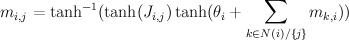
For binary states, update equations become particularly simple.



Here, m_{i,j} is the "message" being sent from node i to node j. If we view message passing as a way of computing marginal conditioned on the evidence, then message {i,j} represents the log-odds that node i is positive, given all the evidence on the other side of of the edge i,j. If our graph has loops, then "other side" of the edge doesn't make sense, but you can use the equations anyway, and this is called "loopy BP".

For binary networks with at most 1 loop, Yair Weiss showed that even though loopy BP may give incorrect probability estimates, highest probability labels under BP will be the same.

Implementation of loopy BP is below. Basically you add up all the messages from neighbours, subtract the message of the target node, then "squash" the message towards zero using ArcTanh[Tanh[J]Tanh[x]] function. Procedure loopyBP takes a matrix of connections, local potential strengths, and returns a function that represents one iteration of BP. Below you see the first few iterations for the graphical model above






To get the final potential at any given node, just add up all the incoming messages. For the graph above, we can plot the probabilities and see that they fall on the correct side of zero after 10 iterations, so that is much smaller computational burden than exact marginalization.




Below you can see the estimates produced by running loopy BP for 200 iterations. The top bar at each node is the actual probability, the bottom bar is the estimated probability using loopy BP. You can see that the feedback makes the estimates overly confident.



For graphs with more than one cycle, loopy BP is no longer guaranteed to converge, or to give MAP labelling when it converges. For instance, here's an animation of loopy BP applied to square Ising lattice with randomly initialized neighbour potentials




Some methods like the Convex-Concave procedure and Generalized Belief Propagation improve on BP's convergence and accuracy.

Mathematica notebook used to produce these figures

Ising model

Ising Models are important for Machine Learning because they are well-studied physical counter-parts of binary valued undirected graphical models. Belief Propagation in such models is equivalent to iteration of the Bethe-Pieirls fixed point equations. Recently Michael Chertkov and Vladimir Chernyak formulated an expression that gave exact expression for the partition function in terms of a local BP solution (slides), and Gómez,Mooij,Kappen followed up by truncating the exact expression and applying it to diagnostic inference task (related slides, approach based on method by Montanari and Rizzo)slides)

While catching up on Ising models, here are a few Ising Model introductory materials I've scanned/scavenged

• Sang Hoon Lee: Introduction to Ising Model and Opinion Dynamics for non-physicists -- basic concept of the Ising model.
  
  
• Rasaiah: Statistical mechanics of strongly interacting systems, chapter from Encyclopedia of Chemical Physics and Physical Chemistry -- solution for 1d Ising model, with and without magnetic field.
  
  
• Dorogovtsev et al: Critical phenomena in complex networks -- Chapter 6 gives algorithms for Ising model, relates to graphical model formalism
  
  
• Salinas: Ising Model, chapter from "Introduction to Statistical Physics" -- Ising model on a lattice, mean field and BP approximation, Curie-Weiss model
  
  

Belief propagation and fixed point iteration

As mentioned in another post belief propagation is a an important algorithm both in probabilistic inference, and statistical thermodynamics. An interesting, and open question both in physics and graphical inference communities is finding the rate at which Belief-Propagation converges for various graphs. Knowing that belief propagation approximately converges after k iterations, would mean that node Y is approximately independent of evidence on node X if the distance between them is k or more, so you could ignore far away away evidence.

Fast convergence would also imply minimum of Bethe free energy approximation to be a good approximation to true free energy (we know that BP fixed points are local minima of Bethe free energy, and also that fast convergence implies fixed points are close together), which means that Bethe free energy approximations are good

We can restrict ourselves to 1 dimensional binary chain model with constant local potentials/evidence

One way to visualize fixed point iteration is through a cob-web plot. Each iteration can be viewed as a horizontal projection to y=x line, then vertical projection to the curve. For instance, here are fixed point iterations for the BP equations of 1d Ising model (equivalent to 2-state hidden markov chain) for weak and strong local potentials.





If we'd like to see how the number of iterations till convergence depends on magnetic field and interaction parameters, we could try approximate the function with a quadratic around fixed point, and compute the number of fixed point iterations needed for that quadratic. However, that by itself is a hard problem. Consider fixed point iterations of the quadratics below



We can replace each plot in the image above by a point that's colored according to how many fixed point iterations were required to converge, keeping same scale but adding some intermediate points we get the diagram below.



You can see the tell-tale signs of chaos in the diagram above, so clearly the general problem of finding convergence rate of fixed point iterations for quadratics is hard.

We can do an analogous plot for the iterations of original BP equation



And similarly coloring the points according to the number of iterations needed to converge we get:



x axis here shows interaction strength between neighbours. You can see with 0 interaction, BP converges in 1 step. Y axis is the strength of evidence. You can see the slowest convergence speed is when there's strong negative corellation between neighbours, or when there's strong positive corellation, and strong negative local evidence. The plot is lopsided because my initial point was 0.5.

This doesn't exhibit the chaotic structure, so in this case reducing the problem to general quadratic actually makes the problem harder.

Mathematica notebook

a step towards open access

Congress recently passed a bill that requires all NIH funded researchers make their papers publically available. If there's no veto, this would require NIH researchers to upload final versions of their papers to PubMed Central

link 1
link 2

Why software libraries aren't reused

Software Libraries and Their Reuse: Entropy, Kolmogorov Complexity, and Zipf’s Law

2,3 universal Turing machine proof disputed

A promising proof of universality of a 2,3 Turing machine (announced here) seems to have stirred some controversy. Vaughan Pratt's post and Todd Rowland's reply

I've recently gone to Northwest Probability Seminar and one topic that came up was Thorp shuffling:

Take a deck of cards, split it in 2 evenly, then proceed to riffle them by dropping card from stack x, followed by card from the other stack, where x could be stack 1 or stack 2 with equal probability. So if we have 4 cards, numbered 1..4, then 1234 will become one of 1324,1342,3124,2142 after one shuffle. How many times should you shuffle until the deck is randomized?

Solving this for n cards has been called the "longest standing open problem in the theory of mixing times".

Since card shuffling is a random walk on a vertex transitive graph, so we could check what that graph looks like.



Mathematica's graph drawing algorithms doesn't take into account special vertex transitive structure, so the graph will looks like a mess.

Going to 3D doesn't help much



One way to discover structure of a matrix is to decompose it into a sum of rank 1 matrices.

Here's the adjacency matrix of the graph above


We can represent it as a sum of following 6 rank-1 matrices.



We can look at the graph corresponding to each of these matrices


This shows all the transitions present in the original graph, but you can see much more structure. In particular, all 6 graphs are isomorphic and bipartite, and the arrows are going only one way between partitions. If we put nodes in each "source" partition into one node, you can see an overall structure of the graph



Finally, we can arrange the nodes in the original graph so that the nodes in the same partition are close together, and here's the result:



Here's the Mathematica notebook I used to produce these figures. Web version

Caveat Lector -- positive definite

There seems to be a difference in definitions of "positive-definite" between pure and applied math literature. For instance:

Linear algebra textbook (Horn and Johnson, 1990):
x^*Ax>0 for all non-zero x
x^* refers to conjugate transpose

Machine Learning textbook (Bishop, 2005)
x'Ax>0 for all non-zero x (real domain is implied)

Mathworld
Re(x^*Ax)>0

The main difference in the definitions is that when restricted to real domain, the first definition also requires that A is symmetric, but the last two don't.

Analysis vs information theory

Here's a problem that could be solved using either analysis or information theory, which approach do you think is easier?

Suppose X_1,X_2,... is an infinite sequence of IID random variables. Let E be an event that's shift invariant, ie, if you take the set of all sequences of Xi's that comprise the event, and shift each sequence, you'll have the same set. For instance "Xi's form a periodic sequence" is a shift-invariant event. Show that P(E) is either 0 or 1.

proof techniques

Many people have seen a copy of this tongue-in-cheek email on proof techniques that's been circulating since the 80's. It' funny because it's true, and here is a couple examples from machine learning literature

• Proof by reference to inaccessible literature, The author cites a simple corollary of a theorem to be found in a privately circulated memoir of the Slovenian Philological Society, 1883.
  
  Consider all the papers citing Vapnik's Theory of Pattern Recognition published by Nauka in 1974. That book is in Russian, and is quite hard to find. For instance it's not indexed in Summit, which includes US West Coast university libraries like Berkeley and University of Washington
  
  
• Proof by forward reference: Reference is usually to a forthcoming paper of the author, which is often not as forthcoming as at first.
  
  I came across a couple of these, which I won't mention because it's a bit embarrassing to the authors
  
  
• Proof by cumbersome notation: Best done with access to at least four alphabets and special symbols.
  
  Of course this is more a matter of habit, but I found this this paper hard to read because of the notation. It uses bold, italic, and caligraphic and fractur alphabets. And if 4 alphabets isn't enough, consult this page to see 9 different alphabets you can use
  

L1 regularization papers this year

Looking at the papers from this summer's machine learning conferences
(AAAI, UAI, IJCAI, ICML,COLT) it seems like there have been a lot of papers on L1 regularization this year. There are at least 3 papers on L1 regularization for structure learning by Koller, Wainwright, Murphy, several papers on minimizing l1 regularized log likelihood by Keerthi, Boyd, Gallen Andrew. A couple of groups are working on "Bayesian Logistic Regression" turns out to be "l1 regularized logistic regression" on closer look (surely Thomas Minka wouldn't approve of such term usage). This year's COLT has one.

Evolutionary Artwork

David Oranshak is using evolutionary algorithms to create aesthetically pleasing artwork


Also, "human vs computer" design awards for 2007

Computers beat humans at face recognition task

The top performing system exhibited better performance than human evaluators when matching faces under varying lighting conditions in NIST large scale face recognition benchmark.

See Figure 8 in
http://face.nist.gov/frvt/frvt2006/FRVT2006andICE2006LargeScaleReport.pdf

matrix-vector multiplication complexity

Suppose A,B are nxn matrices, and x is an nx1 vector. Need to compute M1M2...Mm x where each Mi is either A or B. The straightforward approach is to start multiplying from the right, which takes O(n^2 m) operations. Is it possible to have an O(n^2 m) algorithm that solves the problem above, but has a lower time complexity than the baseline?

The lower bound is O(n^2+m) because that's how long it takes to input the problem. If you could improve on the standard approach, you could solve the problem of inference in Markov-1 hidden markov model with binary observations faster than the Forward algorithm

UCI datasets updated

Looks like UCI website has been updated with some new data, including some sequential/relational datasets

http://archive.ics.uci.edu/beta/datasets.html

HMM's and Linear classifiers

I've across the following question recently -- suppose you have a fully specified Markov-1 Hidden Markov Model with binary observations {Xi} and binary states {Yi}. You observe X1,...,Xn and have to predict Yn. Is the Bayes optimal classifier linear? Empirically, the answer seems to be "yes", but it's not clear to how show it.

---
Update actually looks like they are not linear in general, which can be seen a contour-plot of P(Yn|X1,X2,X3) where each axis parametrizes P(Xi|Yi)

Next 10 years of Structured Learning

ILP 07 had a discussion panel on next 10 years of structured learning. The video is now posted on Video Lectures

Here are couple of things that caught my eye

1. Bernhard Pfahringer -- someone should work on a centralized repository like http://www.kernel-machines.org/, except for structured learning

2. Thomas Dietterich -- need a way to combine benefits of high-performance discriminative learning with semantics of generative models (for the purpose of being able to train various modules separately and then combine them)

3. Pedro Domingos -- current systems (logistic regression, perceptron, SVM) have 1 level of internal structure, need to work out ways to learn multi-tiered compact internal structure effectively

4. Pedro Domingos - - should craft algorithms for which tractable inference is the learning bias -- in other words, the algorithm is explicitly tailored to prefer models that are easy to do inference in

Regularizing with arbitrary quadratic forms

People often fit the model to data by minimizing J(w)+w'Bw where J is the objective function and B is some matrix. Normally people use diagonal or symmetric positive definite matrices for B, but what happens if you use other types?

Here's a Mathematica notebook using Manipulate functionality to let you visualize the shrinkage that happens with different matrices, assuming J(w)'s Hessian is the identity matrix. Drag the locators to modify eigenvectors of B.

One thing to note is that if B is badly conditioned, strange things happen, for instance for some values of w*, they may get pushed away from zero. For negative-definite or indefinite matrices B you may get all w*'s getting shrunk away from zero, or they may get flipped across origin, where w* is argmax_w J(w)

Positive Definite

Indefinite

Negative Definite

Cool Papers at ICML 07

Here are a few that caught my eye:

• Scalable Training of L1-regularized Log-linear ModelsThe main idea is to do L-BFGS in an orthant where the gradient of the L1 loss doesn't change. Each time BFGS tries to step out of that orthant, project it's new point on the old orthant, and figure out the new orthant to explore
  
  
• Discriminative Learning for Differing Training and Test DistributionsIn addition to learning P(Y|X,t1), also learn P(this point is from test data|X). You can do logistic regression to model P(this point is from test data|X,t2), and then weight each point in training set by that value when learning P(Y|X). Alternatively you can learn both distributions simultaneously by maximizing P(Y|X,t1,t2) on test data, which gives even better results
  
  
• On One Method of Non-Diagonal Regularization in Sparse Bayesian Learning Relevance Vector Machine "fits" a diagonal Gaussian prior to data by maximizing P(data|prior).
  In the paper they get a tractable method of fitting Laplace/Gaussian priors with non-diagonal matrices by first transforming parameters to a basis which uncorrelates the parameters at the point of maximum likelihood.
  
  
• Piecewise Pseudolikelihood for Efficient Training of Conditional Random FieldsDoing pseudo-likelihood training (replacing p(y1,y2|x) with p(y1|y2,x)p(y2|y1,x)) on small pieces of the graph (piece-wise training) gives better accuracy than pseudo-likelihood training on the true graph
  
  
• CarpeDiem: an Algorithm for the Fast Evaluation of SSL Classifiers -- a useful trick for doing Viterbi faster -- don't bother computing forward values for nodes which are certain to not be included in the best path. You know a node will not be included in the search path if the a+b+c is smaller than some other forward value on the same level. a+b+c is largest forward value on previous level, b is largest possible transition weight, c is the "emission" weight for that node
  

Machine Learning patents

I found a large number of machine learning related patent applications by doing a few queries on http://www.freepatentsonline.com/

Here are a couple that caught my eye:

• Logistic regression (A machine implemented system that facilitates maximizing probabilities)
  
• Boosting (A computer-implemented process for using feature selection to obtain a strong classifier from a combination of weak classifiers)
  
• Decision tree? (Machine learning by construction of a decision function)
  
• Bayesian Conditional Random Fields -- notably, Tom Minka is missing from the list of inventors
  

The interesting question is what the companies will do with those patents. The best thing they can do is to do nothing with them, which seems to be the case for most patents. The worst thing is they can go after regular users that make implementations of those methods freely available. For instance Xerox forced someone I know to remove a visualization applet from their webpage because the applet used hyperbolic space to visualize graphs, and they have patented this method of visualization. Here are some more worst-case scenarios

Does anyone have any other examples of notable machine learning patents/applications?

Log loss or hinge loss?

Suppose you want to predict binary y given x. You fit a conditional probability model to data and form a classifier by thresholding on 0.5. How should you fit that distribution?

Traditionally people do it by minimizing log-loss on data, which is equivalent to maximum likelihood estimation, but that has the property of recovering the conditional distribution exactly with enough data/modelling freedom. We don't care about exact probabilities, so in some sense it's doing too much work.

Additionally, log-loss minimization may sacrifice classification accuracy if it allows it to model probabilities better.

Here's an example, consider predicting binary y from real valued x. The 4 points give the possible 4 possible x values and their true probabilities. If you model p(y=1|x) as 1/(1+Exp(f_n(x))) where f_n is any n'th degree polynomial.

Take n=2, then minimizing log loss and thresholding on 1/2 produces Bayes-optimal classifier



However, for n=3, the model that minimizes log loss will have suboptimal decision rules for half the data.



Hinge loss is less sensitive to exact probabilities. In particular, minimizer of hinge loss over probability densities will be a function that returns returns 1 over the region where true p(y=1|x) is greater than 0.5, and 0 otherwise. If we are fitting functions of the form above, then once hinge-loss minimizer attains the minimum, adding extra degrees of freedom will never increase approximation error.

Here's example suggested by Olivier Bousquet, suppose your decision boundaries are simple, but the actual probabilities are complicated, how well will hinge loss vs log loss do? Consider the following conditional density




Now use the conditional density functions of the same form as before, find minimizers of both log-loss and hinge loss. Hinge-loss minimization always produces Bayes optimal model for all n>1



When minimizing log-loss, the approximation error starts to increase as the fitter tries to match the exact oscillations in the true probability density function, and ends up overshooting.



Here's the plot of the area on which log loss minimizer produces suboptimal decision rule




Mathematica notebook (web version)

Mathematica 6.0 is out

Mathematica 6.0 is out, touted "The most important advance in the 20-year history of Mathematica"

Among the highly anticipated features is the support for joysticks/gamepads (an XBox version is surely to follow shortly), and the ability to use freehand doodles instead of mathematical symbols in equations (handy when you run out of latin/greek alphabets in your equations)