Loopy Belief propagation

Consider a distribution over 6 binary random variables captured by the structure below.



Red represents -1 potential, green represents +1 potential. More precisely, it's the diagram of the following model, where x's are {-1,1}-valued



We'd like to find the odds of x1 being 1. You could do it by dividing sum of potentials over labellings with x1=1 by corresponding sum over labellings with x1=-1.



In a graph without cycles, such sums can be computed in time linear in the number of nodes by means of dynamic programming. In such cases it reduces to a series of local updates







where evidence (or potential) from each branch is found by marginalizing over the separating variable



For binary states, update equations become particularly simple.



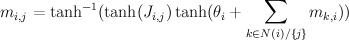
Here, m_{i,j} is the "message" being sent from node i to node j. If we view message passing as a way of computing marginal conditioned on the evidence, then message {i,j} represents the log-odds that node i is positive, given all the evidence on the other side of of the edge i,j. If our graph has loops, then "other side" of the edge doesn't make sense, but you can use the equations anyway, and this is called "loopy BP".

For binary networks with at most 1 loop, Yair Weiss showed that even though loopy BP may give incorrect probability estimates, highest probability labels under BP will be the same.

Implementation of loopy BP is below. Basically you add up all the messages from neighbours, subtract the message of the target node, then "squash" the message towards zero using ArcTanh[Tanh[J]Tanh[x]] function. Procedure loopyBP takes a matrix of connections, local potential strengths, and returns a function that represents one iteration of BP. Below you see the first few iterations for the graphical model above






To get the final potential at any given node, just add up all the incoming messages. For the graph above, we can plot the probabilities and see that they fall on the correct side of zero after 10 iterations, so that is much smaller computational burden than exact marginalization.




Below you can see the estimates produced by running loopy BP for 200 iterations. The top bar at each node is the actual probability, the bottom bar is the estimated probability using loopy BP. You can see that the feedback makes the estimates overly confident.



For graphs with more than one cycle, loopy BP is no longer guaranteed to converge, or to give MAP labelling when it converges. For instance, here's an animation of loopy BP applied to square Ising lattice with randomly initialized neighbour potentials




Some methods like the Convex-Concave procedure and Generalized Belief Propagation improve on BP's convergence and accuracy.

Mathematica notebook used to produce these figures

Ising model

Ising Models are important for Machine Learning because they are well-studied physical counter-parts of binary valued undirected graphical models. Belief Propagation in such models is equivalent to iteration of the Bethe-Pieirls fixed point equations. Recently Michael Chertkov and Vladimir Chernyak formulated an expression that gave exact expression for the partition function in terms of a local BP solution (slides), and Gómez,Mooij,Kappen followed up by truncating the exact expression and applying it to diagnostic inference task (related slides, approach based on method by Montanari and Rizzo)slides)

While catching up on Ising models, here are a few Ising Model introductory materials I've scanned/scavenged

• Sang Hoon Lee: Introduction to Ising Model and Opinion Dynamics for non-physicists -- basic concept of the Ising model.
  
  
• Rasaiah: Statistical mechanics of strongly interacting systems, chapter from Encyclopedia of Chemical Physics and Physical Chemistry -- solution for 1d Ising model, with and without magnetic field.
  
  
• Dorogovtsev et al: Critical phenomena in complex networks -- Chapter 6 gives algorithms for Ising model, relates to graphical model formalism
  
  
• Salinas: Ising Model, chapter from "Introduction to Statistical Physics" -- Ising model on a lattice, mean field and BP approximation, Curie-Weiss model
  
  

Belief propagation and fixed point iteration

As mentioned in another post belief propagation is a an important algorithm both in probabilistic inference, and statistical thermodynamics. An interesting, and open question both in physics and graphical inference communities is finding the rate at which Belief-Propagation converges for various graphs. Knowing that belief propagation approximately converges after k iterations, would mean that node Y is approximately independent of evidence on node X if the distance between them is k or more, so you could ignore far away away evidence.

Fast convergence would also imply minimum of Bethe free energy approximation to be a good approximation to true free energy (we know that BP fixed points are local minima of Bethe free energy, and also that fast convergence implies fixed points are close together), which means that Bethe free energy approximations are good

We can restrict ourselves to 1 dimensional binary chain model with constant local potentials/evidence

One way to visualize fixed point iteration is through a cob-web plot. Each iteration can be viewed as a horizontal projection to y=x line, then vertical projection to the curve. For instance, here are fixed point iterations for the BP equations of 1d Ising model (equivalent to 2-state hidden markov chain) for weak and strong local potentials.





If we'd like to see how the number of iterations till convergence depends on magnetic field and interaction parameters, we could try approximate the function with a quadratic around fixed point, and compute the number of fixed point iterations needed for that quadratic. However, that by itself is a hard problem. Consider fixed point iterations of the quadratics below



We can replace each plot in the image above by a point that's colored according to how many fixed point iterations were required to converge, keeping same scale but adding some intermediate points we get the diagram below.



You can see the tell-tale signs of chaos in the diagram above, so clearly the general problem of finding convergence rate of fixed point iterations for quadratics is hard.

We can do an analogous plot for the iterations of original BP equation



And similarly coloring the points according to the number of iterations needed to converge we get:



x axis here shows interaction strength between neighbours. You can see with 0 interaction, BP converges in 1 step. Y axis is the strength of evidence. You can see the slowest convergence speed is when there's strong negative corellation between neighbours, or when there's strong positive corellation, and strong negative local evidence. The plot is lopsided because my initial point was 0.5.

This doesn't exhibit the chaotic structure, so in this case reducing the problem to general quadratic actually makes the problem harder.

Mathematica notebook

a step towards open access

Congress recently passed a bill that requires all NIH funded researchers make their papers publically available. If there's no veto, this would require NIH researchers to upload final versions of their papers to PubMed Central

link 1
link 2

Why software libraries aren't reused

Software Libraries and Their Reuse: Entropy, Kolmogorov Complexity, and Zipf’s Law