Suppose I have an invertible function $f(x)$. In a perfect world, the following holds
$$x=f(f^{-1}(x))=f^{-1}(f(x))$$
To see what happens in a real world, consider the following
$$D=\left(\begin{matrix}1&1 \\\\ 1&0\end{matrix}\right)^{\otimes\ d}$$
$$f(\mathbf{x})=D\exp (\mathbf{x} D)$$
$f(x)$ maps natural parameters $x$ to mean value parameters $\mu$ in an exponential family over $\{0,1\}^d$
Let $d=6, x=<1/2,1/2,1/2,\ldots,1/2,1>$. Using machine arithmetic you get the following
$$ \|f^{-1}(f(x))-x\|_{\infty}\approx 2.6\times 10^{-15} $$
and
$$\|f(f^{-1}(x))-x\|_{\infty} \approx 0.21$$
Saturday, September 25, 2010
Friday, September 24, 2010
Updated Machine Learning/Statistics blog list
I recently raked the blogosphere for interesting new Machine Learning/math blogs and got a high recall, low precision list of 87, here.
Thursday, September 16, 2010
Dirac integration trick
Suppose X is distributed as n-dimensional Gaussian with 0 mean and concentration matrix $A$ and you need conditional distribution of $P(\mathbf{x}|\mathbf{vx}=\mathbf{0})$ where $\mathbf{v}$ is some unit norm vector. To normalize this density you need to integrate $\exp(-\mathbf{x}'A\mathbf{x})$ over subspace of $\mathbb{R}^n$ orthogonal to $\mathbf{v}$, how do you do it?
Take the Dirac delta function. A nice property is that
$$\int dx \delta(x) f(x) = f(0)$$
Write it in terms of Fourier transform
$$\delta(x)=\int dk\exp(-2\pi i k x)$$
Now we can integrate our Gaussian over whole domain, but multiply by $\delta(\mathbf{v}' \mathbf{x})$ to set to 0 density in regions not orthogonal to $\mathbf{v}$. Changing integration order we get
$$Z_v=\int dk \int d\mathbf{x} \exp(-\mathbf{x}'A\mathbf{x}-2\pi i k \mathbf {v}' \mathbf{x})$$
Second integral is a standard Gaussian integral and can be solved by completing the square (Appendix B, Bishop's "Neural Networks"). The first then becomes another Gaussian integral, with final result
$$Z_v=\left(\frac{\pi^{d-1}} {|A| \mathbf{v'}A^{-1}\mathbf{v}}\right)^\frac{1}{2}$$
Sunday, September 05, 2010
MaxEnt or Bayesian?
Foundations of probabilistic inference is often a subject of much disagreement, with some leading Bayesian sometimes going as far as to say that MaxEnt method doesn't make any sense, and the MaxEnt camp picking on the issue of subjectivity.
The way I see it, MaxEnt and Bayesian approaches are just different ways of using external information to pick a probability distribution.
With Bayesian approach, you are given data and a prior. Bayesian inference then comes out as a natural extension of logic to probabilities. See Ch.1 of Cox's Algebra of Probable Inference for full axiomatic derivation.
With MaxEnt approach, you are given a set of valid probability distributions. You can then justify MaxEnt axiomatically but personally I like the motivation given in Jaynes book, Probability Theory: The Logic of Science (in particular Ch.11).
Roughly speaking, it goes as follows. Suppose we have a distibution $p$ over $d$ outcomes. We say that a sequence of $n$ observations is explained by distribution $p$ if relative counts of outcomes in this sequence match $p$ exactly. The number of sequences matched by $p$ is the following quantity
$$c(p)=\frac{n!}{(np_1)!(np_2)!\cdots (np_d)!}$$
If we have a set of valid distributions $p$, it then makes sense to pick the one with highest $c(p)$ because it'll fit the greatest number of possible future datasets. Approximating $n!$ by $n^n$ we get the following
$$\frac{1}{n}\log c(p)\approx \frac{1}{n}\log \frac{n^n}{(np_1)^{np_1}(np_2)^{np_2}\cdots (np_d)^{np_d}}=H(p)$$
Hence picking distribution with highest H(p) usually means picking the distribution that will be able to explain the most possible observation sequences. Because it's an approximation, there can be exceptions, for instance distributions $(\frac{12}{18},\frac{3}{18},\frac{3}{18})$ and $(\frac{9}{18},\frac{8}{18},\frac{1}{18})$ have equal entropy, but the latter explains 18% more length 18 sequences.
To carry out the inference, Bayesian approach needs to start with a prior, whereas MaxEnt approach needs to start with a set of valid distributions. In practice people often use constant function for prior, and "distributions for which expected feature counts match observed feature counts" for the valid set of distributions.
Note that when dealing with continuous distributions, result of MaxEnt inference depends on the choice of measure over our set of distributions, so I think it's hard to justify in continuous case.
Here are some papers I scanned a while back on foundations of Bayesian and MaxEnt approaches.
Saturday, September 04, 2010
non-asymptotic uses of Central Limit Theorem
Suppose we throw a fair coin n times and estimate it's bias by averaging the number of heads observed. What is the squared error of this estimator?
Using standard binomial identities we can calculate this quantity exactly
$$\sum_{k=0}^n {n\choose k} 2^{-n} (\frac{k}{n}-\frac{1}{2})^2=\frac{1}{4n}$$
Another approach is to use the Central Limit Theorem to approximate exact density with a Gaussian. Using differentiation trick to evaluate the Gaussian integral we get the following estimate of the error
$$\int_{-\infty}^\infty \sqrt{\frac{2}{\pi n}} \exp(-2n(\frac{k}{n}-\frac{1}{2})^2)(\frac{k}{n}-\frac{1}{2})^2 dk=\frac{1}{4n}$$
You can see that using "large-n" approximation in place of exact density gives us the exact result for the error! This hints that Central Limit Theorem could be good for more than just asymptotics.
To see why this approximation gives exact result, rearrange the densities above to get an approximate value of k'th binomial coefficient
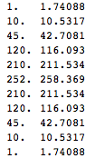
$${n\choose k} \approx \sqrt{\frac{2}{\pi n}} \exp(-2n(\frac{k}{n}-\frac{1}{2})^2) 2^n$$
Below are exact and approximate binomial coefficients for n=10, you can see it's fairly close
This is similar to an approximation we'd get if we used Stirling's approximation. However, Stirling's approximation always overestimates the coefficient, whereas error of this approximation is more evenly distributed. Here's plot of logarithm of error of our approximation and one using Stirling's, top curve is Stirling's approximation.
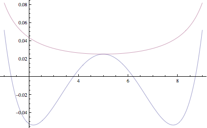
You can see that errors in the estimate due to CLT are sometimes negative and sometimes positive and in the variance calculation above, they happen to cancel out exactly
Using standard binomial identities we can calculate this quantity exactly
$$\sum_{k=0}^n {n\choose k} 2^{-n} (\frac{k}{n}-\frac{1}{2})^2=\frac{1}{4n}$$
Another approach is to use the Central Limit Theorem to approximate exact density with a Gaussian. Using differentiation trick to evaluate the Gaussian integral we get the following estimate of the error
$$\int_{-\infty}^\infty \sqrt{\frac{2}{\pi n}} \exp(-2n(\frac{k}{n}-\frac{1}{2})^2)(\frac{k}{n}-\frac{1}{2})^2 dk=\frac{1}{4n}$$
You can see that using "large-n" approximation in place of exact density gives us the exact result for the error! This hints that Central Limit Theorem could be good for more than just asymptotics.
To see why this approximation gives exact result, rearrange the densities above to get an approximate value of k'th binomial coefficient
$${n\choose k} \approx \sqrt{\frac{2}{\pi n}} \exp(-2n(\frac{k}{n}-\frac{1}{2})^2) 2^n$$
Below are exact and approximate binomial coefficients for n=10, you can see it's fairly close
This is similar to an approximation we'd get if we used Stirling's approximation. However, Stirling's approximation always overestimates the coefficient, whereas error of this approximation is more evenly distributed. Here's plot of logarithm of error of our approximation and one using Stirling's, top curve is Stirling's approximation.
You can see that errors in the estimate due to CLT are sometimes negative and sometimes positive and in the variance calculation above, they happen to cancel out exactly
Subscribe to:
Posts (Atom)