- Hinged tesselation
- Statistics-related Cartoons on stats.SE

- Memorable math paper titles, like Coxeter's "My Graph" (about Coxeter graph).
- Memorable Computer Science paper titles. It includes a series of papers "Functional Programming with Bananas, Lenses, Envelopes and Barbed Wire", and "Seee More through Lenses than Bananas.". Apparently these are functional programming terms
- Annals of Improbable Research

Saturday, January 01, 2011
Happy New Year
Here are some links to start the new year on a light note
Tuesday, December 21, 2010
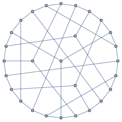
Visualizing 7 dimensional simplex
Suppose we'd like to visualize a set of joint probabilities realizable by distributions of 3 binary variables.
It is a 7 dimensional regular simplex, and we could draw a lower dimensional section of it. There's an infinite number of sections, but there aren't that many *interesting* ones.
As an example, suppose we want to find a good 2 dimensional section of a 3 dimensional regular simplex. It seems reasonable to restrict attention to sections that go through simplex center and two other points, each of which is a vertex or a center of some edge or face. There are just 2 such sections determined up to rotation/reflection
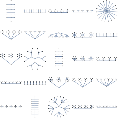
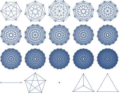
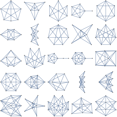
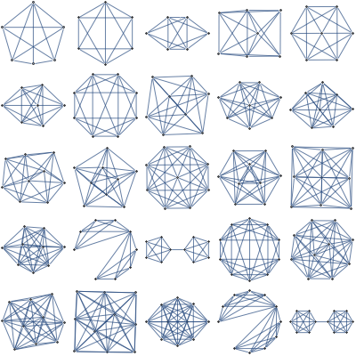
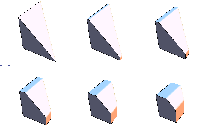
For 7 dimensional simplex, we could similarly take 3 dimensional sections determined by simplex center and 3 points, each a centroid of some set of vertices. This gives 49 distinct shapes, shown below.
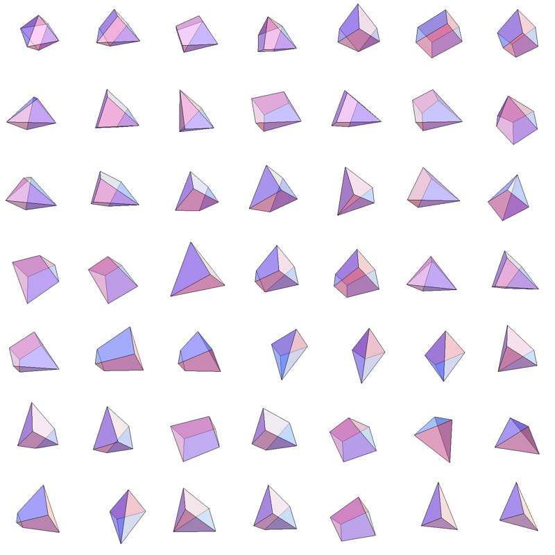
Among those, there's just one section that intersects all 8 faces of the simplex and preserves the underlying symmetry
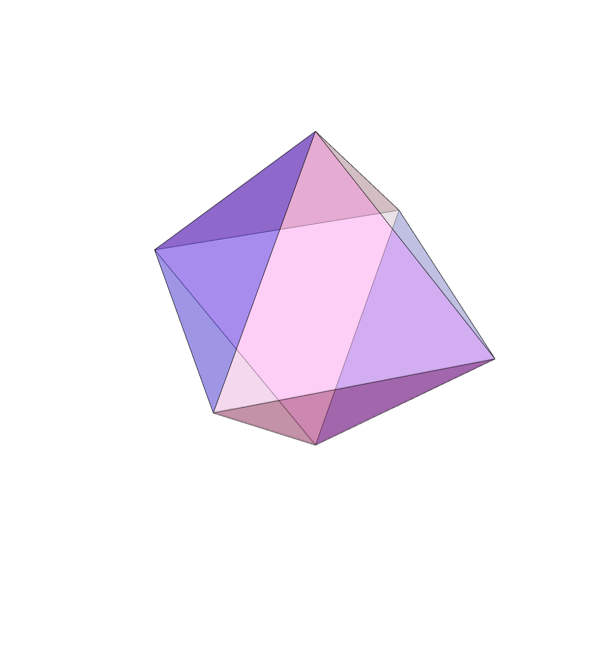
Also known as the regular octahedron.
Implementation details
It is a 7 dimensional regular simplex, and we could draw a lower dimensional section of it. There's an infinite number of sections, but there aren't that many *interesting* ones.
As an example, suppose we want to find a good 2 dimensional section of a 3 dimensional regular simplex. It seems reasonable to restrict attention to sections that go through simplex center and two other points, each of which is a vertex or a center of some edge or face. There are just 2 such sections determined up to rotation/reflection
For 7 dimensional simplex, we could similarly take 3 dimensional sections determined by simplex center and 3 points, each a centroid of some set of vertices. This gives 49 distinct shapes, shown below.
Among those, there's just one section that intersects all 8 faces of the simplex and preserves the underlying symmetry
Also known as the regular octahedron.
Implementation details
Wednesday, December 15, 2010
Computationally nice structures
One approach to solving hard problems is to break them into computationally efficient parts.
For instance, Globerson/Jaakkola do approximate counting by decomposing graph into planar graphs. In each part, the problem reduces to perfect matchings which can be solved efficiently on planar graph. Bouchet/Jordan decompose counting bipartite perfect matchings into much easier problems that count matchings perfect on "one side" of the graph. Sontag/Jaakola solve subproblems on star-shaped subgraphs of original graph, the symmetry of star graph enabling a very fast solution to each subproblem.
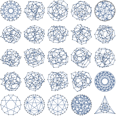
I recently came across graph class database which gives information on thousands of graph classes. It shows dozens (hundreds?) distinct tractable classes for exact maximum independent set, and most of them seem to have unbounded tree width. I haven't heard of most of those classes and would be curious to know how many distinctly interesting algorithms they correspond to
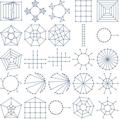
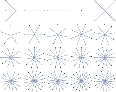
Here are a few computationally nice structures I've seen employed in Machine Learning and Vision literature
Everything is easy via tree decomposition
Almost everything is easy via loopy belief propagation
Easy minimization of submodular functions. Easy counting of certain structures by reduction to perfect matchings.
Easy counting of unweighted local structures
Easy MAP inference with NAND potentials
Very efficient updates for MAP inference
A generalization of line graphs. Easy maximum independent set, and counting by reduction to matchings
Any other useful classes I missed?
Mathematica notebook
For instance, Globerson/Jaakkola do approximate counting by decomposing graph into planar graphs. In each part, the problem reduces to perfect matchings which can be solved efficiently on planar graph. Bouchet/Jordan decompose counting bipartite perfect matchings into much easier problems that count matchings perfect on "one side" of the graph. Sontag/Jaakola solve subproblems on star-shaped subgraphs of original graph, the symmetry of star graph enabling a very fast solution to each subproblem.
I recently came across graph class database which gives information on thousands of graph classes. It shows dozens (hundreds?) distinct tractable classes for exact maximum independent set, and most of them seem to have unbounded tree width. I haven't heard of most of those classes and would be curious to know how many distinctly interesting algorithms they correspond to
Here are a few computationally nice structures I've seen employed in Machine Learning and Vision literature
Upper-bounded tree width
Everything is easy via tree decomposition
Lower-bounded girth
Almost everything is easy via loopy belief propagation
Planar
Easy minimization of submodular functions. Easy counting of certain structures by reduction to perfect matchings.
Complete
Easy counting of unweighted local structures
Perfect
Easy MAP inference with NAND potentials
Star
Very efficient updates for MAP inference
Claw-free
A generalization of line graphs. Easy maximum independent set, and counting by reduction to matchings
Any other useful classes I missed?
Mathematica notebook
Sunday, December 12, 2010
NIPS 2010 highlights
A few "connection to other fields" papers I found interesting
Some interesting applied papers
At least four groups (Bach, Mosci, Jia, Micchelli) had papers on "structured sparsity". Traditional approach to sparse learning is to maximize the number of 0's in the parameter vector. The new idea is to incorporate knowledge on the pattern of 0 values.
Andy Mueller has some more highlights
- Variational Inference over Combinatorial Spaces. Alexandre Bouchard-Cote, Michael Jordan:
Extend variational formulation to upper bound the number of combinatorial structures with global constraints, like perfect matchings and TSP tours. The trick is to represent the space of structures as an intersection of spaces that are tractable to count. For perfect matchings, it is tractable to count edge sets that satisfy perfect matching constraint on one side, so you can represent the total space as intersection of perfect matchings that are "left-legal" and "right-legal". In experiments, the algorithm gave same accuracy for perfect matchings as existing PTAS based on Jerrum's technique, but 10 times faster. - Learning Efficient Markov Networks. Vibhav Gogate, William Webb, Pedro Domingos:
Learn high tree-width models and ensure efficient inference by restricting potential functions to a compact representation as a tree of AND/OR predicates. The problem of learning is reduced to symmetric submodular function minimization which can be done in $O(n^3)$ time with Queyranne's algorithm. For experiments, $O(n^3)$ was too slow, but they give a heuristic which worked to give state-of-the-art results in a practical dataset. - MAP estimation in Binary MRFs via Bipartite Multi-cuts. Sashank Jakkam Reddi, Sunita Sarawagi, Sundar Vishwanathan:
Reduces MAP inference in binary Markov Fields to multi-commodity flow problem - Worst-case bounds on the quality of max-product fixed-points. Meritxell Vinyals, Jesús Cerquides, Alessandro Farinelli, Juan Antonio Rodríguez-Aguilar:
Uses an inequality recently obtained in multi-agent literature to bound difference between true max-marginal and max-product max-marginal in terms of graph structure
Some interesting applied papers
- Segmentation as maximum weight independent set. William Brendel, Sinisa Todorovic:
You want to segment your image into regions, but the initial candidate regions are overlapping fragments. Real segmentations don't have overlaps, turn this into MWIS problem to find good solution satisfying these mutual exclusivity constraints - Efficient Minimization of Decomposable Submodular Functions. Peter Stobbe, Andreas Krause:
Applies some recent techniques from non-smooth optimization to Lovasz extension of submodular function - Optimal Web-Scale Tiering as a Flow Problem. Gilbert Leung, Novi Quadrianto, Alexander Smola, Kostas Tsioutsiouliklis:
Linear integer programming to optimize cache arrangement for 84 million web-pages on Yahoo servers
At least four groups (Bach, Mosci, Jia, Micchelli) had papers on "structured sparsity". Traditional approach to sparse learning is to maximize the number of 0's in the parameter vector. The new idea is to incorporate knowledge on the pattern of 0 values.
Andy Mueller has some more highlights
Sunday, December 05, 2010
Mathematica blog
Most graphics and formulas that appear in this blog were created with help of Mathematica. I'll keep a separate blog with Mathematica tips.
Friday, December 03, 2010
Moving away from traditional peer-review
Common complaint about current publishing model is that sometimes good papers get rejected. A striking example is that David Lowe's SIFT algorithm was rejected multiple times from vision venues. The author then assumed that vision community is not interested, and applied for patent intended promote it just for industrial applications. As a result, what's arguably the most popular key-point detection algorithm is not free to use. This may also say something about limitation of our patent system.
You can see a few more examples in the inaugural issue of Mathematica Rejecta.
Yann LeCun proposes a solution to the problem.
His idea is like non-anonymous stack overflow, where you could search for papers that got several positive reviews, or ones that were positively reviewed by a specific reviewer.
I think the problem is not as serious now as it was before the Internet. Lobachevsky's work was rejected from peer-reviewed journals and might have faced obscurity if not for personal intervention of Gauss.
Today, if your result is obviously important, putting it up on your webpage may end up giving you as much publicity as a publication in a top journal, Ryan Williams latest CS-theoretical result is an example. This approach can also work to screen for errors, as we have seen in the case of Vinay Deolalikar P!=NP paper.
University of Minnesota officially looked into ways of assessing "new forms of scholarship in consideration of academic promotion. Andrew Gelman notices that his most influential papers were published in low ranking journals.
The bottom line is that world is shifting away from the traditional peer-reviewed publication model. Good results don't always need an official stamp of approval to be recognized, and perhaps in 30 years, mentioning the journals where you published at an academic interview will be as bad as coming to a software engineer interview with a heap of Certificates of Proficiency
This reminds me of a faculty candidate that came to interview to our Computer Science department once. He gave a good presentation but didn't get the job. I asked the person in charge of the hiring committee why, the answer was -- "he had too many publications, they couldn't all be good"
Tuesday, November 30, 2010
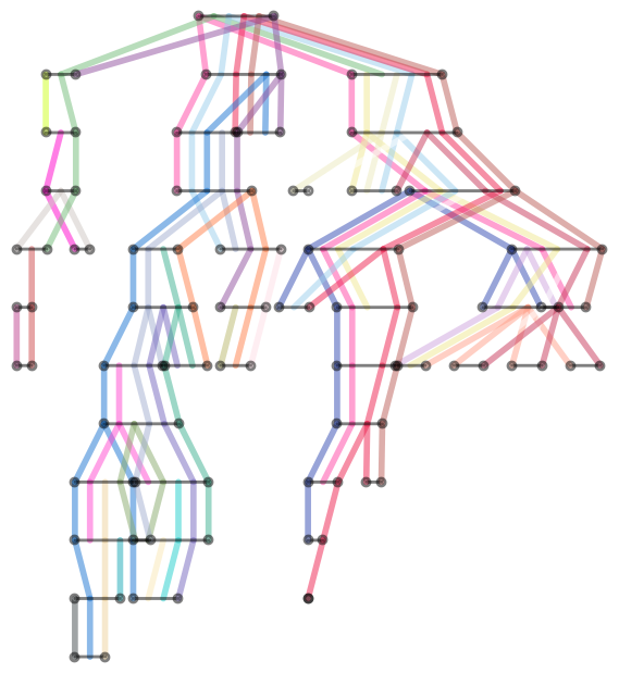
Visualizing Tree Decompositions
In order to do exact probabilistic inference on real life network efficiently, one must find a good Tree Decomposition of the network. This process is known as the Junction Tree algorithm. It's a bit hard to visualize the result, but while browsing tree decomposition graph pages on Wikipedia, I got an idea. Instead of bags with variables, we plot it as a collection of colored strips where each strip corresponds to a variable and Running Intersection property guarantees there will be no breaks.
Here's the result for the width-7 tree decomposition of the moralized Barley network
Mathematica source
Here's the result for the width-7 tree decomposition of the moralized Barley network
Mathematica source
Sunday, November 28, 2010
Springer temporarily opens "Machine Learning" journal
Link here.
If you never heard of the journal "Machine Learning", it used to be number 1 ranked journal in ML, until board of editors resigned and founded the Journal of Machine Learning Research, possibly the greatest success story in open-access publishing
If you never heard of the journal "Machine Learning", it used to be number 1 ranked journal in ML, until board of editors resigned and founded the Journal of Machine Learning Research, possibly the greatest success story in open-access publishing
Friday, November 19, 2010
Prediction competitions
I just came across kaggle.com which is a platform for "s a platform for data prediction competitions." From brief glance, it seems the goal is to automate Netflix-prize-like competitions. It seems four competitions are currently active
Wednesday, November 17, 2010
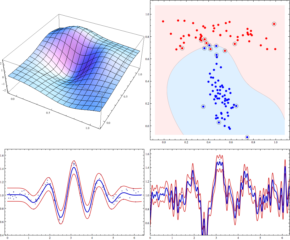
SVM plots
Ulrich Bodenhofer has made some nifty SVM visualization code. One is Mathematica notebooks that takes libSVM model files and visualizes them, another one generates plots of Bayes optimal classifier on some synthetic 2d problems
Tuesday, November 02, 2010
Importance of naming things
Searching for "NIPS" in google blog-search mainly produces posts about nipples, my "CRF" subscription on delicious recently flooded me with links about "Chronic Renal Failure" (apparently a common feline ailment), and you can guess what I got when trying to find Bill Sutherlands "Beautiful Models" book (it's about statistical physics models).
Other unfortunate name choices -- hard-ass (hard as satisfiability, proposed for NP-complete problems before they had a name), Go programming language, hardcore model, Michael Jordan
As a rule of thumb, when coming up with a name for new technique, conference, concept, etc, it should satisfy at least one of two criteria:
- not already be a popular keyword in google
- be funny (ie RODEO ("regularization of derivative expectation operator") as an improvement on the LASSO (least absolute shrinkage and selection operator))
Thursday, October 28, 2010
Sometimes simplest learners are best -- WinnowTag.com experiment
In 1993, R.Holte noted that "Very simple classification rules perform well on most commonly used datasets". His very simple rules are basically binary classifiers that make decision based on value of a single attribute.
In the race for latest and greatest classifiers it's easy to forget that many kinds of classification tasks in 1993 still come up today, so conclusions of Holte's paper still apply.
I came across this effect couple of years ago on a set of document categorization experiments. Folks at WinnowTag wanted me to look into various methods for automatically tagging news/blog items. The idea was that a user manually tags some articles, the system learns and gradually takes over the role of tagging. You can approach it as a straight-forward binary classification task since number of errors represents the number of tag additions/deletions needed from user to fix the tagging.
At first I thought about jumping in and coding some latest and greatest approach for multi-tag labeling like one in from NIPS'04 paper, but as a sanity check, I decided to try existing Weka's classifiers on the dataset.
Nice thing about Weka is that it provides a unified command line interface to all of its classifiers, so you could make a simple Python script like this to run 64 different classifiers on your classification task with default parameters provided by Weka.
4000 hours of EC2 runs later, I got the results. Simplest classifiers like Naive Bayes, OneR (from Holt's paper) made the smallest number of errors. Weka's BayesNet, J48, VotedPerceptron, LibSVM performed as bad or worse as predicting "False" for every tag. Logistic Regression, Neural Networks, AdaboostM1 failed to finish after a day of training.
In retrospect, it makes sense -- in the original dataset there were 35 tags and 5-40 documents per tag, sometimes as small as a couple of sentences, and with the amount of inherent noise in tagging, that's simply not enough data to identify some of the deeper patterns that higher complexity classifiers are made for. In this settings, I wouldn't expect "advanced" classifiers to give a significant improvement over Naive Bayes even after significant tuning of hyper-parameters
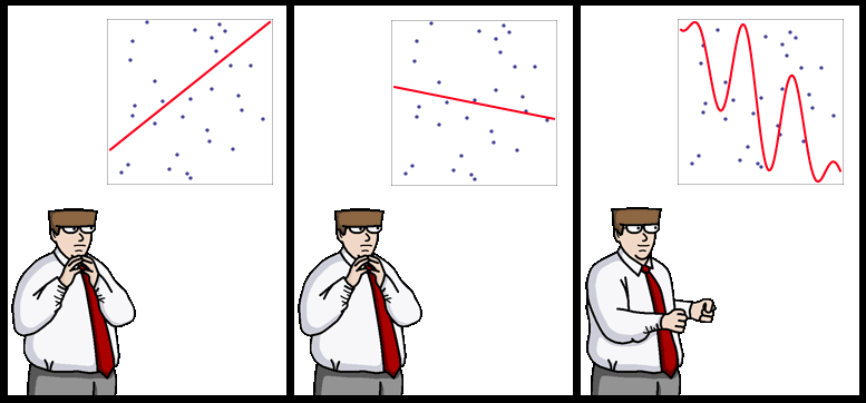
It's been suggested that more data beats better algorithms, but here, I would say that when you have little data/prior knowledge, simplest learners work as well as the most advanced ones.
PS: $1 for the caption to the strip above
Tuesday, October 26, 2010
Times they are a'changin'
Suresh points out that at this year's FOCS, not a single person wanted printed proceedings, whereas few years ago, a third of the audience would ask for printed version.
I see a similar shift happening with technical books. Purists say that you can't beat the convenience of browsing a real book, but I say that you can't beat the convenience of having access to all your books wherever you go. In the last 6 years, I came across about a hundred technical books I considered interesting enough to get an electronic version of, and since publishers didn't provide electronic versions, this often meant me going to the library and scanning the book myself. One of my first blog posts was on the subject of book scanning.
Today, almost 6 years later, I almost never need to use the scanner, because almost every book I need is already available in electronic form, scanned by someone and circulating freely on the Internet. Increasing number of those illegally circulating books are not even scans, but look like bona fide original electronic versions. Number of legally available electronic versions is also increasing, recent examples I came across are Boyd's Convex Optimization, McCallaugh's Tensor Methods in Statistics and Szeliski's Computer Vision: Algorithms and Applications. Times they are a'changin' !
Friday, October 22, 2010
ICML topic trends
David Mimno fit a Dirichlet-multinomial to ICML papers 2004-2008. Seems like "real world" problems are going strong, while boosting took a serious dive
Wednesday, October 13, 2010
Why do we need integrals in Computer Science?
A comment on previous post asked why we need integrals for computer science. One reason is that combinatorial expressions often have representation in terms of integrals. Consider binomial coefficients. We have the following
$${n \choose \frac{n+d}{2}}=\frac{1}{2 \pi} \int_{-\pi}^\pi e^{-\mathbb{i} q d} (2\cos q)^n dq$$
To see where this comes from, consider that $2 \cos x=e^{-\mathbb{i}\pi}+e^{\mathbb{i}\pi}$ is the generating function for number of one step walks starting at 0. Coefficients give number of those walks ending at 1 and -1. Raise it to $n$ and apply inverse Fourier transform to get number of $n$ step walks ending at at $d$, which has an alternative representation in terms of binomial coefficient.
Here's what the result looks like for arbitrary $d$ with $n=10$
Another way to get binomial coefficients is to note that they form coefficients of power of $x$ in expansion of $(1+x)^n$. Use Cauchy's integral formula to recover the coefficient.
We get the following
$${n \choose k} = \frac{1}{2\pi \mathbb{i}}\oint_c \frac{(1+x)^n}{x^{k+1}}$$
Contour integral is counter-clockwise around some contour that encircles the origin.
For instance, you can use the following contour.
Mathematica notebook
Sunday, October 03, 2010
Saturday, October 02, 2010
Universal Laws and Computational Irreducibility
They give opposing perspective -- in the end of speech Stephen Wolfram argues that most processes in universe are "computationally irreducible" and we have no hope to simulating them accurately, whereas Terry Tao's article gives examples of many things in real world obeying a small set of simple laws
Saturday, September 25, 2010
Order Matters
Suppose I have an invertible function $f(x)$. In a perfect world, the following holds
$$x=f(f^{-1}(x))=f^{-1}(f(x))$$
To see what happens in a real world, consider the following
$$D=\left(\begin{matrix}1&1 \\\\ 1&0\end{matrix}\right)^{\otimes\ d}$$
$$f(\mathbf{x})=D\exp (\mathbf{x} D)$$
$f(x)$ maps natural parameters $x$ to mean value parameters $\mu$ in an exponential family over $\{0,1\}^d$
Let $d=6, x=<1/2,1/2,1/2,\ldots,1/2,1>$. Using machine arithmetic you get the following
$$ \|f^{-1}(f(x))-x\|_{\infty}\approx 2.6\times 10^{-15} $$
and
$$\|f(f^{-1}(x))-x\|_{\infty} \approx 0.21$$
Friday, September 24, 2010
Updated Machine Learning/Statistics blog list
I recently raked the blogosphere for interesting new Machine Learning/math blogs and got a high recall, low precision list of 87, here.
Thursday, September 16, 2010
Dirac integration trick
Suppose X is distributed as n-dimensional Gaussian with 0 mean and concentration matrix $A$ and you need conditional distribution of $P(\mathbf{x}|\mathbf{vx}=\mathbf{0})$ where $\mathbf{v}$ is some unit norm vector. To normalize this density you need to integrate $\exp(-\mathbf{x}'A\mathbf{x})$ over subspace of $\mathbb{R}^n$ orthogonal to $\mathbf{v}$, how do you do it?
Take the Dirac delta function. A nice property is that
$$\int dx \delta(x) f(x) = f(0)$$
Write it in terms of Fourier transform
$$\delta(x)=\int dk\exp(-2\pi i k x)$$
Now we can integrate our Gaussian over whole domain, but multiply by $\delta(\mathbf{v}' \mathbf{x})$ to set to 0 density in regions not orthogonal to $\mathbf{v}$. Changing integration order we get
$$Z_v=\int dk \int d\mathbf{x} \exp(-\mathbf{x}'A\mathbf{x}-2\pi i k \mathbf {v}' \mathbf{x})$$
Second integral is a standard Gaussian integral and can be solved by completing the square (Appendix B, Bishop's "Neural Networks"). The first then becomes another Gaussian integral, with final result
$$Z_v=\left(\frac{\pi^{d-1}} {|A| \mathbf{v'}A^{-1}\mathbf{v}}\right)^\frac{1}{2}$$
Sunday, September 05, 2010
MaxEnt or Bayesian?
Foundations of probabilistic inference is often a subject of much disagreement, with some leading Bayesian sometimes going as far as to say that MaxEnt method doesn't make any sense, and the MaxEnt camp picking on the issue of subjectivity.
The way I see it, MaxEnt and Bayesian approaches are just different ways of using external information to pick a probability distribution.
With Bayesian approach, you are given data and a prior. Bayesian inference then comes out as a natural extension of logic to probabilities. See Ch.1 of Cox's Algebra of Probable Inference for full axiomatic derivation.
With MaxEnt approach, you are given a set of valid probability distributions. You can then justify MaxEnt axiomatically but personally I like the motivation given in Jaynes book, Probability Theory: The Logic of Science (in particular Ch.11).
Roughly speaking, it goes as follows. Suppose we have a distibution $p$ over $d$ outcomes. We say that a sequence of $n$ observations is explained by distribution $p$ if relative counts of outcomes in this sequence match $p$ exactly. The number of sequences matched by $p$ is the following quantity
$$c(p)=\frac{n!}{(np_1)!(np_2)!\cdots (np_d)!}$$
If we have a set of valid distributions $p$, it then makes sense to pick the one with highest $c(p)$ because it'll fit the greatest number of possible future datasets. Approximating $n!$ by $n^n$ we get the following
$$\frac{1}{n}\log c(p)\approx \frac{1}{n}\log \frac{n^n}{(np_1)^{np_1}(np_2)^{np_2}\cdots (np_d)^{np_d}}=H(p)$$
Hence picking distribution with highest H(p) usually means picking the distribution that will be able to explain the most possible observation sequences. Because it's an approximation, there can be exceptions, for instance distributions $(\frac{12}{18},\frac{3}{18},\frac{3}{18})$ and $(\frac{9}{18},\frac{8}{18},\frac{1}{18})$ have equal entropy, but the latter explains 18% more length 18 sequences.
To carry out the inference, Bayesian approach needs to start with a prior, whereas MaxEnt approach needs to start with a set of valid distributions. In practice people often use constant function for prior, and "distributions for which expected feature counts match observed feature counts" for the valid set of distributions.
Note that when dealing with continuous distributions, result of MaxEnt inference depends on the choice of measure over our set of distributions, so I think it's hard to justify in continuous case.
Here are some papers I scanned a while back on foundations of Bayesian and MaxEnt approaches.
Saturday, September 04, 2010
non-asymptotic uses of Central Limit Theorem
Suppose we throw a fair coin n times and estimate it's bias by averaging the number of heads observed. What is the squared error of this estimator?
Using standard binomial identities we can calculate this quantity exactly
$$\sum_{k=0}^n {n\choose k} 2^{-n} (\frac{k}{n}-\frac{1}{2})^2=\frac{1}{4n}$$
Another approach is to use the Central Limit Theorem to approximate exact density with a Gaussian. Using differentiation trick to evaluate the Gaussian integral we get the following estimate of the error
$$\int_{-\infty}^\infty \sqrt{\frac{2}{\pi n}} \exp(-2n(\frac{k}{n}-\frac{1}{2})^2)(\frac{k}{n}-\frac{1}{2})^2 dk=\frac{1}{4n}$$
You can see that using "large-n" approximation in place of exact density gives us the exact result for the error! This hints that Central Limit Theorem could be good for more than just asymptotics.
To see why this approximation gives exact result, rearrange the densities above to get an approximate value of k'th binomial coefficient
$${n\choose k} \approx \sqrt{\frac{2}{\pi n}} \exp(-2n(\frac{k}{n}-\frac{1}{2})^2) 2^n$$
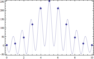
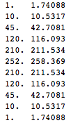
Below are exact and approximate binomial coefficients for n=10, you can see it's fairly close
This is similar to an approximation we'd get if we used Stirling's approximation. However, Stirling's approximation always overestimates the coefficient, whereas error of this approximation is more evenly distributed. Here's plot of logarithm of error of our approximation and one using Stirling's, top curve is Stirling's approximation.
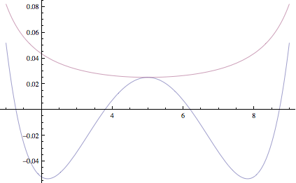
You can see that errors in the estimate due to CLT are sometimes negative and sometimes positive and in the variance calculation above, they happen to cancel out exactly
Using standard binomial identities we can calculate this quantity exactly
$$\sum_{k=0}^n {n\choose k} 2^{-n} (\frac{k}{n}-\frac{1}{2})^2=\frac{1}{4n}$$
Another approach is to use the Central Limit Theorem to approximate exact density with a Gaussian. Using differentiation trick to evaluate the Gaussian integral we get the following estimate of the error
$$\int_{-\infty}^\infty \sqrt{\frac{2}{\pi n}} \exp(-2n(\frac{k}{n}-\frac{1}{2})^2)(\frac{k}{n}-\frac{1}{2})^2 dk=\frac{1}{4n}$$
You can see that using "large-n" approximation in place of exact density gives us the exact result for the error! This hints that Central Limit Theorem could be good for more than just asymptotics.
To see why this approximation gives exact result, rearrange the densities above to get an approximate value of k'th binomial coefficient
$${n\choose k} \approx \sqrt{\frac{2}{\pi n}} \exp(-2n(\frac{k}{n}-\frac{1}{2})^2) 2^n$$
Below are exact and approximate binomial coefficients for n=10, you can see it's fairly close
This is similar to an approximation we'd get if we used Stirling's approximation. However, Stirling's approximation always overestimates the coefficient, whereas error of this approximation is more evenly distributed. Here's plot of logarithm of error of our approximation and one using Stirling's, top curve is Stirling's approximation.
You can see that errors in the estimate due to CLT are sometimes negative and sometimes positive and in the variance calculation above, they happen to cancel out exactly
Monday, August 30, 2010
New Machine Learning blog
By Frank Nielsen, with focus on information geometry, http://blog.informationgeometry.org/
Sunday, August 15, 2010
Method of Types
After following some discussions on overflow sites, I re-read Shannon/Cover's coverage of method of types, and want to summarize it here because of how useful and underappreciated it is.
A type or type class is basically an empirical distribution for a sequence of n independent events. For instance, suppose we flip coin n=2 times. We have 3 type classes, all heads, all tails, one head/one tail. Size of the type class is the number of sequences in that class. Here, two of our classes have size 1 and "one head/one tail" has size 2.
Since the number of types grows polynomially with n, while number of observation sequences grows exponentially, some type classes end up getting an exponential number of sequences. Since constants of exponential growth are different for different types, probability mass ends up getting concentrated in a small number of types and several important properties follow from this concentration behavior.
In particular, Thomas/Cover use method of types to formalize and prove the following statements in Chapter 12 of "Information Theory and Statistics" (1991).
Resources
A type or type class is basically an empirical distribution for a sequence of n independent events. For instance, suppose we flip coin n=2 times. We have 3 type classes, all heads, all tails, one head/one tail. Size of the type class is the number of sequences in that class. Here, two of our classes have size 1 and "one head/one tail" has size 2.
Since the number of types grows polynomially with n, while number of observation sequences grows exponentially, some type classes end up getting an exponential number of sequences. Since constants of exponential growth are different for different types, probability mass ends up getting concentrated in a small number of types and several important properties follow from this concentration behavior.
In particular, Thomas/Cover use method of types to formalize and prove the following statements in Chapter 12 of "Information Theory and Statistics" (1991).
- Probability of hypothesis E under distribution P is determined by the probability of closest member of E to P (Sanov's theorem)
- To test whether data x was generated by p or q, it's sufficient to only look at the ratio of probabilities of x under p and under q (Neyman-Pearson lemma)
- When data is generated by p or q and you are trying to tell which one it is from data, probability of making a mistake for an optimal classifier is bounded by exp(-n max(KL(p,q),KL(q,p)). A tighter bound is to use KL(x,p)=KL(x,q) where x is the "halfway point" between distributions (Chernoff's theorem)
Rodriguez says it outperforms BIC and AIC by orders of magnitude
- Thomas, Cover "Information Theory and Statistics"
- Csiszar, Shields Notes on Information Theory and Statistics
Tuesday, August 10, 2010
Interesting Stack Exchanges
As I discovered recently, stack exchanges can be pretty fun, informative (and time consuming!) way to discuss issues related to machine learning. Here are some relevant ones I found
There's also stack exchange for Machine Learning and Computer Vision that are in proposal phase. Any interesting ones I missed?
Machine Learning stack exchange is right now undergoing definition. Please go and vote on interesting questions to help define it as a research-level discussion forum
- Statistical Analysis
- Math
- Natural Language Processing
- High-level math (non-research level questions will be closed)
There's also stack exchange for Machine Learning and Computer Vision that are in proposal phase. Any interesting ones I missed?
Machine Learning stack exchange is right now undergoing definition. Please go and vote on interesting questions to help define it as a research-level discussion forum
Friday, August 21, 2009
Robust OCR in video
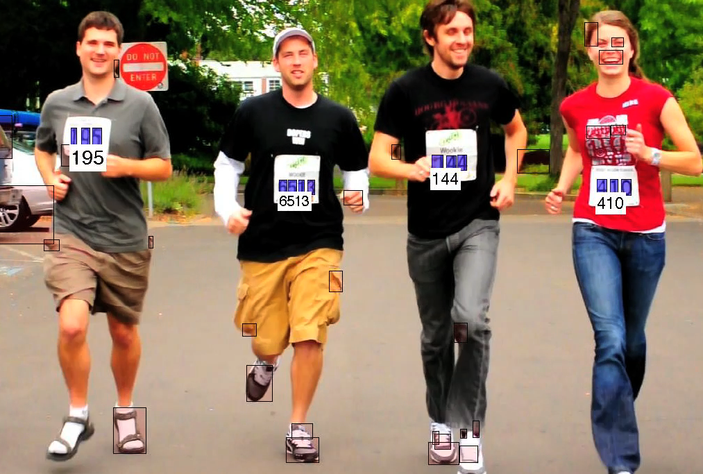
I used the "Robust OCR dataset" below to make a system for reading runner bibs in video. Standard ML techniques give fairly good results without much tweaking -- AdaBoost with stumps to go through all connected components (in thresholded image) and generate potential candidates, SVM/Gaussian kernel to classify those candidates into digits. Here's a screenshot and a video of this system in action.
Video
Video
Wednesday, August 05, 2009
New Robust OCR dataset

I've collected this dataset for a project that involves automatically reading bibs in pictures of marathons and other races. This dataset is larger than robust-reading dataset of ICDAR 2003 competition with about 20k digits and more uniform because it's digits-only. I believe it is more challenging than the MNIST digit recognition dataset.
I'm now making it publicly available in hopes of stimulating progress on the task of robust OCR. Use it freely, with only requirement that if you are able to exceed 80% accuracy, you have to let me know ;)
The dataset file contains raw data (images), as well as Weka-format ARFF file for simple set of features.
For completeness I include matlab script used to for initial pre-processing and feature extraction, Python script to convert space-separated output into ARFF format. Check "readme.txt" for more details.
Dataset
Sunday, July 12, 2009
machine vision resource
This seems to be a fairly comprehensive vision bibliography. I found a few articles on text localization there that I didn't find through scholar/citation following
http://www.visionbib.com/bibliography/contents.html
http://www.visionbib.com/bibliography/contents.html
Tuesday, April 01, 2008
Update
I've started a new job at MyStrands.com, looking at mining financial data.
I also applied to Wolfram Research at the same time, but they were too slow to reply. As part of WRI application, I've put together some prior work, I think these are good examples of the things you can use Mathematica for
I also applied to Wolfram Research at the same time, but they were too slow to reply. As part of WRI application, I've put together some prior work, I think these are good examples of the things you can use Mathematica for
Monday, February 11, 2008
Which DPI to use for scanning papers?
Here's a side to side comparison of 150 vs. 300 vs. 600 DPI scan viewed at 400% magnification. On a local library scanner, 600 DPI black-and-white takes twice as slow to scan as 300 DPI, without significant improvement in quality
Wednesday, February 06, 2008
Strategies for organizing literature
Newton once wrote to Hooke: "If I have seen further it is by standing on the shoulders of giants". It's true nowdays more than ever, and since there's such a huge volume of literature that is electronically searchable, the hard part isn't finding previous work, but remembering where you have found it.
Here's the strategy I use, which relies mainly on CiteULike and Google Desktop, what are some others?
I do similar thing with books, in addition to scanning every technical book that I spend more than a couple of hours reading. With double-sided scans, you can average 4 seconds per page, so well worth the time investment. In addition, book scanning has a kind of meditation effect.
To find some result, ideally I remember the author or tag you put it under, then I use CiteULike search feature. If that fails, use Google Desktop to search through pdf's and web history.
What strategy do you use?
Here's the strategy I use, which relies mainly on CiteULike and Google Desktop, what are some others?
- Use Slogger and "Save As" to save every webpage and pdf I look at, put the pdf's online for ease of access and sharing.
- For more important papers, add an entry to CiteULike with a small comment
- When common themes emerge (like resistance networks or self-avoiding walk trees), go over papers in that area and make sure they share a tag or group of tags
- For papers that are revisited, use "Notes" section for that paper in CiteULike to save page numbers of every important formula or statement in the paper.
- Finally, once a particular theme comes up often enough, review all the papers in that topic, write a mini-summary, put it in the "Notes" section of the oldest paper in that category
I do similar thing with books, in addition to scanning every technical book that I spend more than a couple of hours reading. With double-sided scans, you can average 4 seconds per page, so well worth the time investment. In addition, book scanning has a kind of meditation effect.
To find some result, ideally I remember the author or tag you put it under, then I use CiteULike search feature. If that fails, use Google Desktop to search through pdf's and web history.
What strategy do you use?
Friday, February 01, 2008
Cool formula
Pi comes up in the most unexpected places. Here's an application to walk counting that involves it.
Suppose you have a chain of length n. How many walks of length k are there on the chain? For instance, for a chain of length 5, there are 5 paths of length 0 (start at each vertex and don't go anywhere), 8 of length 1 (traverse each edge either left-right or right-left), 14 of length 2 (8 walks that change direction once, 6 walks that don't change direction) etc.
Curiously enough, there's an explicit formula for this
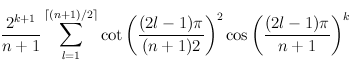
For example, to find the number of walks of length 2 in a chain of length 5, plug n=5, k=2 into formula above, and get
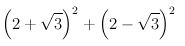
Which is 14.
Notebook, web version
Suppose you have a chain of length n. How many walks of length k are there on the chain? For instance, for a chain of length 5, there are 5 paths of length 0 (start at each vertex and don't go anywhere), 8 of length 1 (traverse each edge either left-right or right-left), 14 of length 2 (8 walks that change direction once, 6 walks that don't change direction) etc.
Curiously enough, there's an explicit formula for this
For example, to find the number of walks of length 2 in a chain of length 5, plug n=5, k=2 into formula above, and get
Which is 14.
Notebook, web version
Monday, January 28, 2008
Russian Captcha revisited
A few weeks ago , I brought up a Russian CAPTCHA that asks to find resistance between end-points in a version of Wheatstone bridge in order to access a forum
There's been some discussion of this problem on Reasonable Deviations blog, with Vladimir Zacharov writing up a general solution for this circuit using two Kirchhoff's (Kirkhoff) laws and one Ohm's law directly .
For larger circuits, this approach gets exponentially more tedious since you get an equation for every loop in the circuit. But apparently you can ignore most of them and look only at "fundamental loops".
An alternative approach is to use one Kirchhoff law and one Ohm's law. Note that:
1) Current across an edge is proportional to voltage drop divided by resistance
2) Net current at each node is 0, (not counting external current)
Hence, for net current at i'th node we get
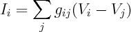
Here g's are conductances on edges. This is just a set of linear equations, so you can rewrite them as

where L is the combinatorial Laplacian of the graph with conductances being edge weights. We inject 1 Amp at node 1 (A), extract 1 Amp at node 4 (B), and solve for voltages.
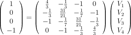
Use your favourite method to solve this linear system. For instance, the following is a solution:
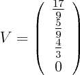
Since current is 1, voltage drop is the same as resistance, hence 17/9 is the answer.
Linear resistor networks turn out to be an amazingly rich subject with connections to many other areas, as can be seen from other ways of solving this problem
- Combinatorics 1: add an edge from 1 to 4 with conductance 1. Resistance is the weighted sum of spanning trees containing new edge divided by the weighted sum of all spanning trees (weighted by product of edge conductances). Formula 4.27 of Wu
- Combinatorics 2: resistance is the determinant of combinatorial Laplacian with 1st/4th row/column removed divided by determinant of said Laplacian with 1st column/row removed. Formula 6 of Bapat and 4.34 of Wu
- Probability Theory 1: Resistance is 1/(cd) where c is conductance of node 1 (sum of incoming edge conductances), d is the probability of random walker starting at node 1 reaching node 4 before coming back to node 1, with node transition probabilities defined by formula 12 in Klein. Formula 13 of Klein
- Probability Theory 2: Add an edge from 1 to 4 with conductance 1. Resistance is the odds of random spanning tree on the graph containing this edge, where probability of each spanning tree is proportional to the product of edge conductances. Follows from formula 4.27 of Wu
- Markov Chain simulation: create a Markov chain with 1 and 4 being trapping states, and transition probabilities defined in previous method. Start with all probability in state 1, let the mass escape once, then simulate Markov chain till convergence. Resistance is 1 divided by mass in node 4 after convergence. Section 1.2.6 of Doyle
- Circuit transformation rules: use star-triangle, parallel and series laws to simplify the circuit to a single resistor. Page 44 of Bollobas. Note that two of these transformation rules have an analogue in graphical models, sections 4.4,4.5 of Sokal.
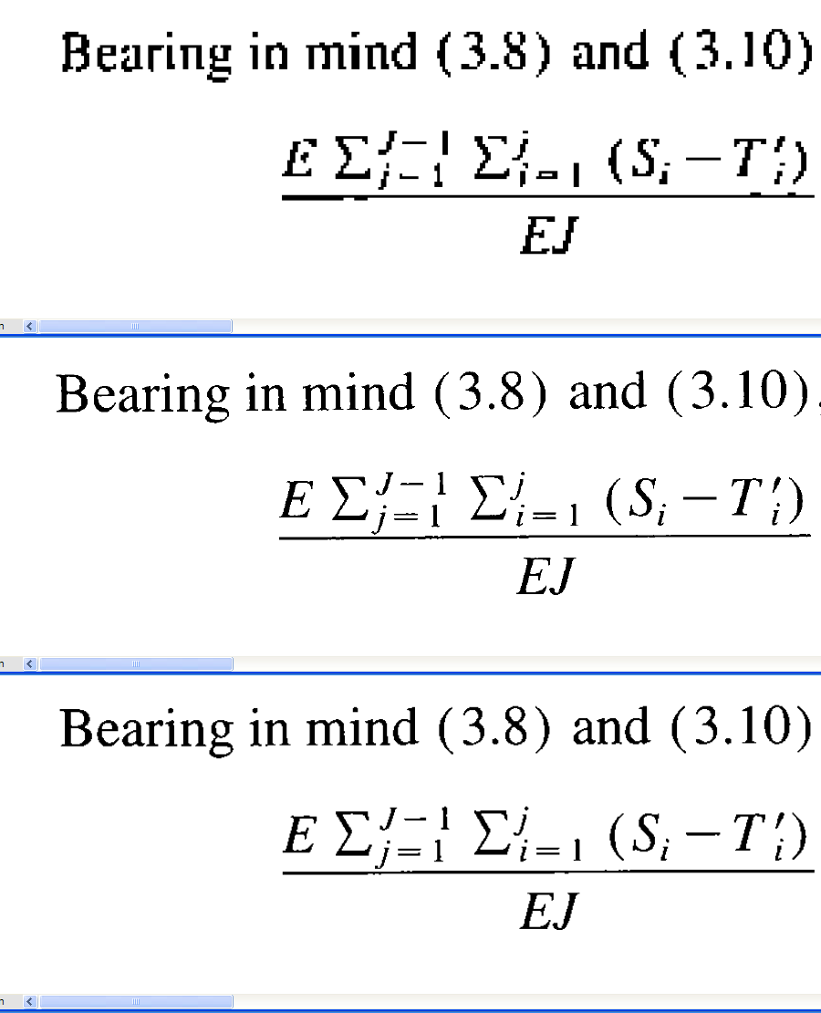
- Optimization Theory: Resistance is R in the following
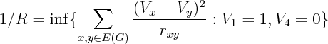 Corollary 5, Chapter 9 of Bollobas
Friday, January 25, 2008
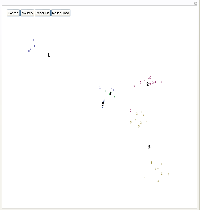
Expectation Maximization for Gaussian Mixtures demo
I was going to post this to Wolfram's Demonstrations website, but then I realized it doesn't fit some technical format limitations, so I'm posting it here.
notebook
It's a demonstration of Expectation-Maximization algorithm, you need Mathematica or free Mathematica Player to run it.
Expectation-Maximization algorithm tries to find centers of clusters in the data. It first assigns each point to some random cluster, each cluster center to random position on the plane, then iterates E and M steps. E-step updates cluster center to be the mean of all datapoints assigned to that cluster, M-step updates each datapoint to be assigned to the cluster whose center is closest to this datapoint. Bold numbers indicate current cluster centers, small numbers indicate datapoints and their current cluster assignment. You can view it as a method of finding approximate maximum likelihood fit of a Gaussian mixture with fixed number of Gaussians and identity covariance matrix. Press "E-step" and "M-step" in alternation to see the algorithm in action.
Thursday, January 17, 2008
Maximum entropy with skewness constraint
Maximum entropy principle is the idea that we should should pick a distribution maximizing entropy subject to certain constraints. Many known distributions come out in this way, such as Gamma, Poisson, Normal, Beta, Exponential, Geometric, Cauchy, log-normal, and others. In fact, there's a close connection between maxent distributions and exponential families -- Darmois-Koopman-Pitman theorem promises that all positive distributions with finite sufficient statistics correspond to exponential families. Recall that exponential families are families that are log-linear in the space of parameters, so in a sense, exponential families are analogous to vector spaces -- whereas vector space is closed under addition, exponential family is closed under multiplication.
After you pick the form of your constraints, the maxent distribution is determined by the value of the constraints. So in this sense, constraint values serve as sufficient statistics, hence by DKP theorem, result must lie in the exponential family determined by form of the constraints.
You can use Lagrange multipliers (see my previous post) to maximize entropy subject to moment constraints. This works to get Normal distribution and Exponential, but if you introduce skewness constraints you get distribution of the form exp(ax+bx^2+cx^3)/Z, which fails to normalize unless c=0, so what went wrong?
This is due to a technical point which doesn't matter for deriving most distributions -- correspondence between maxent and exponential family distributions only holds for distributions that are strictly positive. Also, entropy maximization subject to moment constraints is valid only if non-negativity constraints are inactive. In certain cases, like this one, you must also include nonnegativity constraints, and then the solution fails to have a nice closed form.
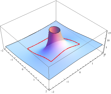
Suppose we maximize entropy in a distribution with 6 bins in the interval [-1,1] with constraints that mean=0, variance=0.3 and skewness=0. In addition to normalization constraint, this leaves a 2 dimensional space of valid distributions, and we can plot the space of valid (nonnegative) distributions, along with their entropy.
Now suppose we change skewness constraint to be 0.15 The new plot is below.
You can see that the maximum entropy solution lies right on the edge of the space of valid distributions, hence the nonnegativity constraint must be active at this point.
To get a sense what the maxent solution might look like, we can discretize the distribution, and do constrained optimization to find a solution. Below is the solution for 20 bins, variance=0.4 and skewness=0.23
I tried various values of positive skewness, and that seems to be a general form -- distribution is 0 for positive x's except for a single spike at largest allowable x, for negative x's there's a Gaussian-like hump.
References:
-- Mathematica notebook, web version
-- Justification of MaxEnt from statistical point of view by Tishby/Tichochinsky
After you pick the form of your constraints, the maxent distribution is determined by the value of the constraints. So in this sense, constraint values serve as sufficient statistics, hence by DKP theorem, result must lie in the exponential family determined by form of the constraints.
You can use Lagrange multipliers (see my previous post) to maximize entropy subject to moment constraints. This works to get Normal distribution and Exponential, but if you introduce skewness constraints you get distribution of the form exp(ax+bx^2+cx^3)/Z, which fails to normalize unless c=0, so what went wrong?
This is due to a technical point which doesn't matter for deriving most distributions -- correspondence between maxent and exponential family distributions only holds for distributions that are strictly positive. Also, entropy maximization subject to moment constraints is valid only if non-negativity constraints are inactive. In certain cases, like this one, you must also include nonnegativity constraints, and then the solution fails to have a nice closed form.
Suppose we maximize entropy in a distribution with 6 bins in the interval [-1,1] with constraints that mean=0, variance=0.3 and skewness=0. In addition to normalization constraint, this leaves a 2 dimensional space of valid distributions, and we can plot the space of valid (nonnegative) distributions, along with their entropy.
Now suppose we change skewness constraint to be 0.15 The new plot is below.
You can see that the maximum entropy solution lies right on the edge of the space of valid distributions, hence the nonnegativity constraint must be active at this point.
To get a sense what the maxent solution might look like, we can discretize the distribution, and do constrained optimization to find a solution. Below is the solution for 20 bins, variance=0.4 and skewness=0.23
I tried various values of positive skewness, and that seems to be a general form -- distribution is 0 for positive x's except for a single spike at largest allowable x, for negative x's there's a Gaussian-like hump.
References:
-- Mathematica notebook, web version
-- Justification of MaxEnt from statistical point of view by Tishby/Tichochinsky
Wednesday, December 26, 2007
Russian CAPTCHA
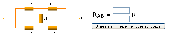
Here's an innovative CAPTCHA I came across when trying to register for a forum at http://lib.mipt.ru/?spage=reg_user
You have to enter resistance between A and B in the diagram below. Can you do it?
You have to enter resistance between A and B in the diagram below. Can you do it?
Monday, December 17, 2007
Sampling doubly stochastic matrices
Stochastic matrices are easy to get -- just normalize the rows. Doubly stochastic matrices require more work -- simply normalizing columns/rows will not converge may take few dozen iterations to converge. One approach that works is to do constrained optimization, finding closest (in least squared sense) doubly stochastic matrix to given matrix. Another approach is to start with a permutation matrix and follow a Markov chain that modifies 4 elements randomly at each step in a way that keeps the matrix doubly stochastic. Here is the implementation of these two methods in Mathematica (notebook in the same directory)
http://www.yaroslavvb.com/research/qr/doubly-stochastic/doubly-stochastic.html
As Jeremy pointed out, Birkhoff's theorem provides necessary and sufficient conditions for a matrix to be doubly stochastic -- it must be a convex combination of permutation matrices. It seems hard to sample from the set of valid convex combinations though. For instance, here's a set of 3 dimensional slices through the set of valid convex combinations for 3x3 matrices (there are 6 permutation matrices, so the space is 5 dimensional).
Update: here's the updated notebook with 2 more algorithms, suggested by Dr.Teh and Jeremy below. Turns out that sampling random convex combinations is fairly easy -- almost all the time uniformly sampled convex combination will produce a doubly-stochastic matrix. However, matrices end up looking pretty uniform
http://www.yaroslavvb.com/research/qr/doubly-stochastic/doubly-stochastic3.html
Sunday, November 25, 2007
Loopy Belief propagation
Consider a distribution over 6 binary random variables captured by the structure below.
Red represents -1 potential, green represents +1 potential. More precisely, it's the diagram of the following model, where x's are {-1,1}-valued

We'd like to find the odds of x1 being 1. You could do it by dividing sum of potentials over labellings with x1=1 by corresponding sum over labellings with x1=-1.
In a graph without cycles, such sums can be computed in time linear in the number of nodes by means of dynamic programming. In such cases it reduces to a series of local updates

where evidence (or potential) from each branch is found by marginalizing over the separating variable
For binary states, update equations become particularly simple.
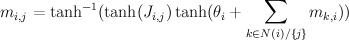
Here, m_{i,j} is the "message" being sent from node i to node j. If we view message passing as a way of computing marginal conditioned on the evidence, then message {i,j} represents the log-odds that node i is positive, given all the evidence on the other side of of the edge i,j. If our graph has loops, then "other side" of the edge doesn't make sense, but you can use the equations anyway, and this is called "loopy BP".
For binary networks with at most 1 loop, Yair Weiss showed that even though loopy BP may give incorrect probability estimates, highest probability labels under BP will be the same.
Implementation of loopy BP is below. Basically you add up all the messages from neighbours, subtract the message of the target node, then "squash" the message towards zero using ArcTanh[Tanh[J]Tanh[x]] function. Procedure loopyBP takes a matrix of connections, local potential strengths, and returns a function that represents one iteration of BP. Below you see the first few iterations for the graphical model above
To get the final potential at any given node, just add up all the incoming messages. For the graph above, we can plot the probabilities and see that they fall on the correct side of zero after 10 iterations, so that is much smaller computational burden than exact marginalization.
Below you can see the estimates produced by running loopy BP for 200 iterations. The top bar at each node is the actual probability, the bottom bar is the estimated probability using loopy BP. You can see that the feedback makes the estimates overly confident.
For graphs with more than one cycle, loopy BP is no longer guaranteed to converge, or to give MAP labelling when it converges. For instance, here's an animation of loopy BP applied to square Ising lattice with randomly initialized neighbour potentials
Some methods like the Convex-Concave procedure and Generalized Belief Propagation improve on BP's convergence and accuracy.
Mathematica notebook used to produce these figures
Red represents -1 potential, green represents +1 potential. More precisely, it's the diagram of the following model, where x's are {-1,1}-valued
We'd like to find the odds of x1 being 1. You could do it by dividing sum of potentials over labellings with x1=1 by corresponding sum over labellings with x1=-1.
In a graph without cycles, such sums can be computed in time linear in the number of nodes by means of dynamic programming. In such cases it reduces to a series of local updates
where evidence (or potential) from each branch is found by marginalizing over the separating variable
For binary states, update equations become particularly simple.
Here, m_{i,j} is the "message" being sent from node i to node j. If we view message passing as a way of computing marginal conditioned on the evidence, then message {i,j} represents the log-odds that node i is positive, given all the evidence on the other side of of the edge i,j. If our graph has loops, then "other side" of the edge doesn't make sense, but you can use the equations anyway, and this is called "loopy BP".
For binary networks with at most 1 loop, Yair Weiss showed that even though loopy BP may give incorrect probability estimates, highest probability labels under BP will be the same.
Implementation of loopy BP is below. Basically you add up all the messages from neighbours, subtract the message of the target node, then "squash" the message towards zero using ArcTanh[Tanh[J]Tanh[x]] function. Procedure loopyBP takes a matrix of connections, local potential strengths, and returns a function that represents one iteration of BP. Below you see the first few iterations for the graphical model above
To get the final potential at any given node, just add up all the incoming messages. For the graph above, we can plot the probabilities and see that they fall on the correct side of zero after 10 iterations, so that is much smaller computational burden than exact marginalization.
Below you can see the estimates produced by running loopy BP for 200 iterations. The top bar at each node is the actual probability, the bottom bar is the estimated probability using loopy BP. You can see that the feedback makes the estimates overly confident.
For graphs with more than one cycle, loopy BP is no longer guaranteed to converge, or to give MAP labelling when it converges. For instance, here's an animation of loopy BP applied to square Ising lattice with randomly initialized neighbour potentials
Some methods like the Convex-Concave procedure and Generalized Belief Propagation improve on BP's convergence and accuracy.
Mathematica notebook used to produce these figures
Friday, November 09, 2007
Ising model
Ising Models are important for Machine Learning because they are well-studied physical counter-parts of binary valued undirected graphical models. Belief Propagation in such models is equivalent to iteration of the Bethe-Pieirls fixed point equations. Recently Michael Chertkov and Vladimir Chernyak formulated an expression that gave exact expression for the partition function in terms of a local BP solution (slides), and Gómez,Mooij,Kappen followed up by truncating the exact expression and applying it to diagnostic inference task (related slides, approach based on method by Montanari and Rizzo)slides)
While catching up on Ising models, here are a few Ising Model introductory materials I've scanned/scavenged
While catching up on Ising models, here are a few Ising Model introductory materials I've scanned/scavenged
- Sang Hoon Lee: Introduction to Ising Model and Opinion Dynamics for non-physicists -- basic concept of the Ising model.
- Rasaiah: Statistical mechanics of strongly interacting systems, chapter from Encyclopedia of Chemical Physics and Physical Chemistry -- solution for 1d Ising model, with and without magnetic field.
- Dorogovtsev et al: Critical phenomena in complex networks -- Chapter 6 gives algorithms for Ising model, relates to graphical model formalism
- Salinas: Ising Model, chapter from "Introduction to Statistical Physics" -- Ising model on a lattice, mean field and BP approximation, Curie-Weiss model
Thursday, November 08, 2007
Belief propagation and fixed point iteration
As mentioned in another post belief propagation is a an important algorithm both in probabilistic inference, and statistical thermodynamics. An interesting, and open question both in physics and graphical inference communities is finding the rate at which Belief-Propagation converges for various graphs. Knowing that belief propagation approximately converges after k iterations, would mean that node Y is approximately independent of evidence on node X if the distance between them is k or more, so you could ignore far away away evidence.
Fast convergence would also imply minimum of Bethe free energy approximation to be a good approximation to true free energy (we know that BP fixed points are local minima of Bethe free energy, and also that fast convergence implies fixed points are close together), which means that Bethe free energy approximations are good
We can restrict ourselves to 1 dimensional binary chain model with constant local potentials/evidence
One way to visualize fixed point iteration is through a cob-web plot. Each iteration can be viewed as a horizontal projection to y=x line, then vertical projection to the curve. For instance, here are fixed point iterations for the BP equations of 1d Ising model (equivalent to 2-state hidden markov chain) for weak and strong local potentials.
If we'd like to see how the number of iterations till convergence depends on magnetic field and interaction parameters, we could try approximate the function with a quadratic around fixed point, and compute the number of fixed point iterations needed for that quadratic. However, that by itself is a hard problem. Consider fixed point iterations of the quadratics below
We can replace each plot in the image above by a point that's colored according to how many fixed point iterations were required to converge, keeping same scale but adding some intermediate points we get the diagram below.
You can see the tell-tale signs of chaos in the diagram above, so clearly the general problem of finding convergence rate of fixed point iterations for quadratics is hard.
We can do an analogous plot for the iterations of original BP equation
And similarly coloring the points according to the number of iterations needed to converge we get:
x axis here shows interaction strength between neighbours. You can see with 0 interaction, BP converges in 1 step. Y axis is the strength of evidence. You can see the slowest convergence speed is when there's strong negative corellation between neighbours, or when there's strong positive corellation, and strong negative local evidence. The plot is lopsided because my initial point was 0.5.
This doesn't exhibit the chaotic structure, so in this case reducing the problem to general quadratic actually makes the problem harder.
Mathematica notebook
Subscribe to:
Posts (Atom)