How to patent an algorithm in the US

Today I got Google Alert today on the following pending patent -- Belief Propagation for Generalized Matching. I like to stay up on Belief Propagation literature, so I took a closer look. The PDF linked gives a fairly detailed explanation of belief propagation for solving matching problems, including pseudocode which is very detailed, looking like an excerpt of a C program. Appendix A seems to be an expanded version of a paper which appeared in NIPS 2008 workshop

A pecularity of the US patent system is that patents on algorithms are not allowed, yet algorithms are frequently patented. A few years ago when I blogged on the issue of patents in Machine Learning, I didn't know the specifics, but now, having gone through the process, I know a bit more.

When filing an algorithm patent, patent lawyer will tell you to remove every instance of the word "algorithm" and replace it with some other word. This seems to be necessary for getting the patent through.

So, in the patent above, belief propagation algorithm is referred to as "belief propagation system". In the whole application, word "system" occurs 114 times, whereas "algorithm" occurs 1 time, in reference to a competing approach.

Another thing the patent lawyer will probably ask for is lots and lots of diagrams. I'm guessing that diagrams serve as further evidence that your algorithm is a "system" and not merely an algorithm. There are only so many useful diagrams you can have, so at some point you may find yourself pulling diagrams from thin ar and thinking "why am I doing this?" (but then remembering that it's because of the bonus). In the industry, a common figure seems to be $5000 for a patent that goes through. If a company doesn't have bonus structure, they may use other means to pressure employees into patent process. (note, patent above was filed through a university)

As a result, these kinds of patents end up with vacuous diagrams.

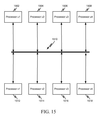
For instance, In the patent above, there are 17 figures, and a few of them don't seem to convey any useful information. The one below is illustrating the "plurality of belief propagation processors connected to a bus"


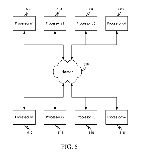
And this one is one is to illustrate belief propagation processors connected to a network


Finally when I saw the following diagram, I first thought it was there to illustrate BP update formula, which involves adding and multiplying numbers



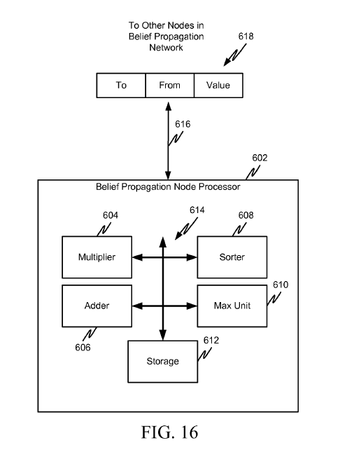
But it's not even tenuously connected to the rest of the patent. 604 is supposed to be "computer readable media", 606 is a "link that couples media to the network", 608 is the "network" for aforementioned "link" and "media". 616 and 618 are not referenced.

This doesn't actually matter because nobody really reads the patent anyway. The most important part of getting the patent through is having a patent lawyer on the case who can frame it in the right format and handle communication with the patent office. The process for regular (non-expedited) patents can take five years and the total cost can exceed $50,000.

As to why an organization would spend so much time and money on a patent that might not even be enforceable by virtue of being an algorithm patent -- patents have intrinsic value. Once patent clears the patent office, a patent is an asset which can be sold or traded and as a result increases company worth. You can sell rights to pending patents before they are granted which makes the actual content of the patent even less important

Generalized Distributive Law

With regular distributive law you can do things like

$$\sum_{x_1,x_2,x_3} \exp(x_1 + x_2 + x_3)=\sum_{x_1} \exp x_1 \sum_{x_2} \exp x_2 \sum_{x_3} \exp x_3$$

This breaks the original large sum into 3 small sums which can be computed independently.

A more realistic scenario requires factorization into overlapping parts. For instance take the following

$$\sum_{x1,x2,x3,x_4,x_5} \exp(x_1 x_2 + x_2 x_3 + x_3 x_4+x_4 x_5)$$

You can't use directly apply distributive law here. Naive evaluation of the sum is exponential in the number of variables, however this problem can be solved in time linear in the number of variables.

Consider the following factorization
$$\sum_{x1,x2} \exp x_1 x_2 \left( \sum_{x_3} \exp x_2 x_3 \left( \sum_{x_4} \exp x_3 x_4 \left( \sum_{x_5} \exp x_4 x_5 \right) \right) \right) $$

Now note that when computing inner sums, naive approach results in same sum being recomputed many times. Save those shared pieces and you get an algorithm that's quadratic in number of variable values and linear in number of variables

Viterbi and Forward-Backward are specific names of this kind of dynamic programming for chain structured sums as above.

To consider tree-structured sum, take a problem of counting independent sets in a tree-structured graph. In this case we can use the following factorization




This is the first step of the recursion and you can repeat it until your pieces have tractable size.

Now for a general case of non-tree-structured graph, consider the sum below

$$\sum_{x1,x2,x3,x_4,x_5} \exp( x_1 x_2 + x_2 x_3 + x_3 x_4+x_4 x_5 + x_5 x_1 )$$

Here, variables form a loop, so regular tree recursion like Viterbi does not apply. However, this sum can be found efficiently, linear in the number of variables, and cubically in the number of variable values. I have more in depth explanation of decomposing problems like above in an answer on cstheory site but the basic idea is similar to the approach with independent sets -- fix some variables and recurse on subparts.

This kind of general factorization has been re-invented many times and is known as Generalized Distributive Law, tree-decomposition, junction tree, clique tree, partial k-tree, and probably a few other names.


Notebook

Cluster decomposition and variational counting

Suppose we want to count the number of independent sets in a graph below.



There are 9 independent sets.


Because the graphs are disjoint we could simplify the task by counting graphs in each connected component separately and multiplying the result



Variational approach is one way of extending this decomposition idea to connected graphs.

Consider the problem of counting independent sets in the following graph.


There are 7 independent sets. Let $x_i=1$ indicate that node $i$ is occupied, and $P(x_1,x_2,x_3,x_4)$ be a uniform distribution over independent sets, meaning it is either 1/7 or 0 depending whether $x_1,x_2,x_3,x_4$ forms an independent set

Entropy of uniform distribution over $n$ independent sets distribution is $H=-\log(1/n)$, hence $n=\exp H$, so to find the number of independent sets just find the entropy of distribution $P$ and exponentiate it.

We can represent P as follows

$$P(x_1,x_2,x_3,x_4)=\frac{P_a(x_1,x_2,x_3)P_b(x_1,x_3,x_4)}{P_c(x_1,x_3)}$$

Entropy of P similarly factorizes

$$H=H_a + H_b - H_c$$

Once you have $P_A$, $P_B$ and $P_C$ representing our local distributions of our factorization, we can forget the original graph and compute the number of independent sets from entropies of these factors

To find factorization of $P$ into $P_a,P_b$, and $P_c$ minimize the following objective

$$KL(\frac{P_a P_b}{P_c},P)$$

This is KL-divergence between our factorized representation and original representation. Message passing schemes like cluster belief propagation can be derived as one approach of solving this minimization problem. In this case, cluster belief propagation takes 2 iterations to find the minimum of this objective. Note that the particular form of distance is important. We could reverse the order and instead minimize $KL(P,P_a P_b/P_c)$ and while this makes sense from approximation stand-point, minimizing reversed form of KL-divergence is generally intractable.


This decomposition is sufficiently rich that we can model P exactly using proper choice of $P_a,P_b$ and $P_c$, so the minimum of our objective is 0, and our entropy decomposition is exact.

Now, the number of independent sets using decomposition above factorizes as
$$n=\exp H=\frac{\exp H_a \exp H_b}{\exp H_c} = \frac{\left(\frac{7}{2^{4/7}}\right)^2}{\frac{7}{2\ 2^{1/7}}} = \frac{4.75 \times 4.75}{3.17}=7$$

Our decomposition can be schematically represented as the following cluster graph



We have two regions and we can think of our decomposition as counting number of independent sets in each region, then dividing by number of independent sets in the vertex set shared by pair of connected regions. Note that region A gets "4.75 independent sets" so this is not as intuitive as decomposition into connected components


Here's another example of graph and its decomposition.





Using 123 to refer to $P(x_1,x_2,x_3)$ the formula representing this decomposition is as follows

$$\frac{124\times 236\times 2456 \times 4568 \times 478\times 489}{24\times 26 \times 456 \times 48 \times 68}$$

There are 63 independent sets in this graph, and using decomposition above the count decomposes as follows:

$$63=\frac{\left(\frac{21\ 3^{5/7}}{2\ 2^{19/21} 5^{25/63}}\right)^2 \left(\frac{3\ 21^{1/3}}{2^{16/21} 5^{5/63}}\right)^4}{\frac{21\ 3^{3/7}}{2\ 2^{1/7} 5^{50/63}} \left(\frac{3\ 21^{1/3}}{2\ 2^{3/7} 5^{5/63}}\right)^4}$$


Finding efficient decomposition that models distribution exactly requires that graph has small tree-width. This is not the case for many graphs, such as large square grids, but we can apply the same procedure to get cheap inexact decomposition.

Consider the following inexact decomposition of our 3x3 grid



Corresponding decomposition has 4 clusters and 4 separators, and the following factorization formula

$$\frac{1245\times 2356 \times 4578 \times 5689}{25\times 45 \times 56 \times 58}$$

We can use minimization objective as before to find the parameters of this factorization. Since original distribution can not be exactly represented in this factorization, result will be approximate, unlike previous two example.

Using message-passing to solve the variational problem takes about 20 iterations to converge, to an estimate of 46.97 independent sets




To try various decompositions yourself, unzip the archive and look at usage examples in indBethe3-test.nb

Notebooks

Junction trees in numerical analysis

There's a neat connection between Cholesky factorization and graph triangulations -- graph corresponding to Cholesky factorization of a sparse matrix is precisely the triangulation of the sparse matrix (when viewed as a graph) using canonical elimination ordering.

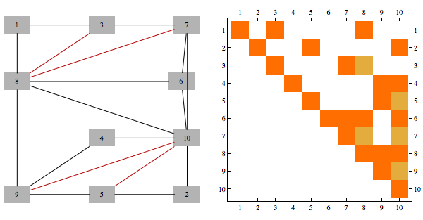
Here's an example of a matrix (corresponding to the graph with black edges only), and its Cholesky factorization. We triangulate the graph by any pairs of neighbors of v which have higher index than v, for every v. Extra edges added in this way correspond to extra non-zero entries in Cholesky decomposition of the original matrix. Different color edges/matrix entries correspond to non-zero entries in Cholesky factorization not present in original matrix



Furthermore, junction tree we get using min-fill heuristic of a graph is same structure as what is used to perform Cholesky factorization using parallel multi-frontal method

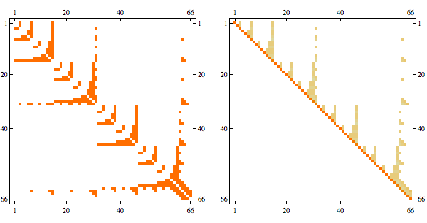
Here's a chordal matrix in perfect order and its Cholesky factorization


The fact that Cholesky factorization has the same sparsity structure as the original matrix confirms that its a chordal matrix in perfect elimination order

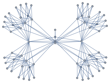
Here's the graph representation of the matrix


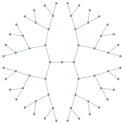
Junction tree decomposition of this graph reveals the following clique structure


High branching structure of decomposition means that Cholesky factorization can be highly parallelized, in particular, the very last step of Cholesky decomposition of this matrix in minfill order consists of 32 independent tasks that can be done in parallel.

I packaged together some Mathematica code for these kinds of tasks