Russian Captcha revisited

A few weeks ago , I brought up a Russian CAPTCHA that asks to find resistance between end-points in a version of Wheatstone bridge in order to access a forum

There's been some discussion of this problem on Reasonable Deviations blog, with Vladimir Zacharov writing up a general solution for this circuit using two Kirchhoff's (Kirkhoff) laws and one Ohm's law directly .

For larger circuits, this approach gets exponentially more tedious since you get an equation for every loop in the circuit. But apparently you can ignore most of them and look only at "fundamental loops".

An alternative approach is to use one Kirchhoff law and one Ohm's law. Note that:
1) Current across an edge is proportional to voltage drop divided by resistance
2) Net current at each node is 0, (not counting external current)

Hence, for net current at i'th node we get



Here g's are conductances on edges. This is just a set of linear equations, so you can rewrite them as



where L is the combinatorial Laplacian of the graph with conductances being edge weights. We inject 1 Amp at node 1 (A), extract 1 Amp at node 4 (B), and solve for voltages.



Use your favourite method to solve this linear system. For instance, the following is a solution:



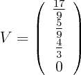
Since current is 1, voltage drop is the same as resistance, hence 17/9 is the answer.

Linear resistor networks turn out to be an amazingly rich subject with connections to many other areas, as can be seen from other ways of solving this problem

• Combinatorics 1: add an edge from 1 to 4 with conductance 1. Resistance is the weighted sum of spanning trees containing new edge divided by the weighted sum of all spanning trees (weighted by product of edge conductances). Formula 4.27 of Wu
  
  
• Combinatorics 2: resistance is the determinant of combinatorial Laplacian with 1st/4th row/column removed divided by determinant of said Laplacian with 1st column/row removed. Formula 6 of Bapat and 4.34 of Wu
  
  
• Probability Theory 1: Resistance is 1/(cd) where c is conductance of node 1 (sum of incoming edge conductances), d is the probability of random walker starting at node 1 reaching node 4 before coming back to node 1, with node transition probabilities defined by formula 12 in Klein. Formula 13 of Klein
  
  
• Probability Theory 2: Add an edge from 1 to 4 with conductance 1. Resistance is the odds of random spanning tree on the graph containing this edge, where probability of each spanning tree is proportional to the product of edge conductances. Follows from formula 4.27 of Wu
  
  
• Markov Chain simulation: create a Markov chain with 1 and 4 being trapping states, and transition probabilities defined in previous method. Start with all probability in state 1, let the mass escape once, then simulate Markov chain till convergence. Resistance is 1 divided by mass in node 4 after convergence. Section 1.2.6 of Doyle
  
  
• Circuit transformation rules: use star-triangle, parallel and series laws to simplify the circuit to a single resistor. Page 44 of Bollobas. Note that two of these transformation rules have an analogue in graphical models, sections 4.4,4.5 of Sokal.
  
  
• Optimization Theory: Resistance is R in the following Corollary 5, Chapter 9 of Bollobas
  

Expectation Maximization for Gaussian Mixtures demo

I was going to post this to Wolfram's Demonstrations website, but then I realized it doesn't fit some technical format limitations, so I'm posting it here.

notebook

It's a demonstration of Expectation-Maximization algorithm, you need Mathematica or free Mathematica Player to run it.

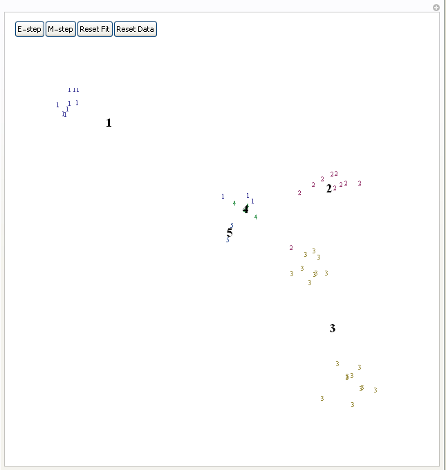
Expectation-Maximization algorithm tries to find centers of clusters in the data. It first assigns each point to some random cluster, each cluster center to random position on the plane, then iterates E and M steps. E-step updates cluster center to be the mean of all datapoints assigned to that cluster, M-step updates each datapoint to be assigned to the cluster whose center is closest to this datapoint. Bold numbers indicate current cluster centers, small numbers indicate datapoints and their current cluster assignment. You can view it as a method of finding approximate maximum likelihood fit of a Gaussian mixture with fixed number of Gaussians and identity covariance matrix. Press "E-step" and "M-step" in alternation to see the algorithm in action.

Maximum entropy with skewness constraint

Maximum entropy principle is the idea that we should should pick a distribution maximizing entropy subject to certain constraints. Many known distributions come out in this way, such as Gamma, Poisson, Normal, Beta, Exponential, Geometric, Cauchy, log-normal, and others. In fact, there's a close connection between maxent distributions and exponential families -- Darmois-Koopman-Pitman theorem promises that all positive distributions with finite sufficient statistics correspond to exponential families. Recall that exponential families are families that are log-linear in the space of parameters, so in a sense, exponential families are analogous to vector spaces -- whereas vector space is closed under addition, exponential family is closed under multiplication.

After you pick the form of your constraints, the maxent distribution is determined by the value of the constraints. So in this sense, constraint values serve as sufficient statistics, hence by DKP theorem, result must lie in the exponential family determined by form of the constraints.

You can use Lagrange multipliers (see my previous post) to maximize entropy subject to moment constraints. This works to get Normal distribution and Exponential, but if you introduce skewness constraints you get distribution of the form exp(ax+bx^2+cx^3)/Z, which fails to normalize unless c=0, so what went wrong?

This is due to a technical point which doesn't matter for deriving most distributions -- correspondence between maxent and exponential family distributions only holds for distributions that are strictly positive. Also, entropy maximization subject to moment constraints is valid only if non-negativity constraints are inactive. In certain cases, like this one, you must also include nonnegativity constraints, and then the solution fails to have a nice closed form.

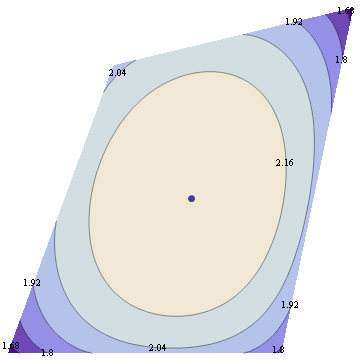
Suppose we maximize entropy in a distribution with 6 bins in the interval [-1,1] with constraints that mean=0, variance=0.3 and skewness=0. In addition to normalization constraint, this leaves a 2 dimensional space of valid distributions, and we can plot the space of valid (nonnegative) distributions, along with their entropy.



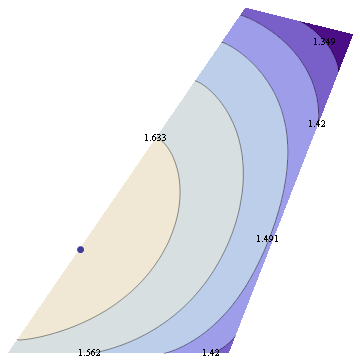
Now suppose we change skewness constraint to be 0.15 The new plot is below.


You can see that the maximum entropy solution lies right on the edge of the space of valid distributions, hence the nonnegativity constraint must be active at this point.

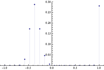
To get a sense what the maxent solution might look like, we can discretize the distribution, and do constrained optimization to find a solution. Below is the solution for 20 bins, variance=0.4 and skewness=0.23



I tried various values of positive skewness, and that seems to be a general form -- distribution is 0 for positive x's except for a single spike at largest allowable x, for negative x's there's a Gaussian-like hump.

References:

-- Mathematica notebook, web version
-- Justification of MaxEnt from statistical point of view by Tishby/Tichochinsky