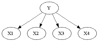
To see that both logistic regression and naive bayes classifier consider the same hypothesis space we can rewrite Naive Bayes density as follows (restricting attention to binary domain):

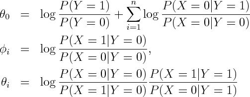
where
Alternatively you can get exponential family parametrization from the observation that Naive Bayes model has no unshielded colliders, so undirected model obtained by dropping the arrows is equivalent on the set of positive densities.
From here you can rewrite it as product of conditional and marginal distributions
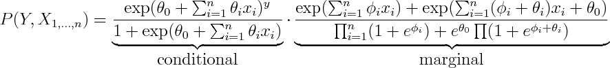
You can see that the conditional term is equivalent to logistic regression, so every possible conditional density that can be modelled by logistic regression can be modelled by Naive Bayes by setting \phi's aribrarily.
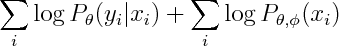
So both logistic regression and Naive Bayes have the same hypothesis space, but optimize different objective functions. In particular logistic regression maximizes
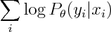
whereas Naive Bayes maximizies
You can see that the second term involves both phis and thetas, so conditional and marginal likelihoods are coupled. If empirical density is realizable by our model, then this coupling doesn't matter -- both conditional and marginal terms can achieve their respective maxima so Naive Bayes and Logistic Regression will produce the same estimate. However that not necessarily true when empirical density is unrealizable -- you may have to compromise between achieving high conditional likelihood and high marginal likelihood.
To get a generatively trained model that is identical to conditionally trained Naive Bayes, Minka suggests treating parameters in conditional and joint as separate sets.
So now we can introduce n new parameters so that conditional and marginal densities become decoupled.

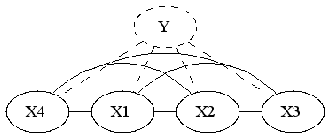
It's interesting to see what is the new marginal density of our model. The marginal density marginalizes out Y. Since Y is the only separator in original graph, the resulting graph will be fully connected.
So if we were to restrict attention to linear exponential families, we'd have to introduce 2^n features. I'm wondering if it's possible to infer that fact by looking at the form of the density. You'd have to show that the size of sufficient statistic is at least 2^n, or alternatively show that the smallest linear space that embeds the unnormalized log densities has dimension 2^n
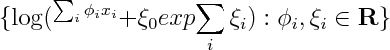
If x_i are real or complex valued, one could show that the smallest linear space that embeds the set above has to be infinite dimensional, by noting that since log(1+exp(ax)) has singularities at i pi a, so one can always construct linearly independent elements by choosing a accordingly. I wonder, are there similar tricks that would work for discrete x?
(derivations)