The Key Theorem of the Learning Theory

The Key Theorem of the Learning Theory is what Vapnik calls his theorem (for instance here) that gives the necessary conditions for the Empirical Risk Minimization principle to be consistent.
The important equation is the following:



Here I'll explain the parts of the formula using the following motivating example:
Suppose our true distribution is a normal distribution with unit variance, centered at 0, and we estimate its mean from data using method of maximum likelihood. This falls into domain of Empirical Risk Minimization because it's equivalent to finding unit variance normal distribution which minimizes empirical log-loss. If this method is consistent, then our maximum likelihood estimate of the mean will be correct in the limit


In order for the theorem to apply, we need to do make sure that we can put a bound on the loss incurred by functions in our hypothesis space, so here, make an additional restriction that our fitted normals must have mean between -100 and 100.

Here's what parts of the equation stand for

1.

l is the size of our training set

2.

a is the parameter that indexes our probability distributions, in this case, it's mean of our fitted Normal. Lambda is it's domain, in this case,


3.

This is the actual risk incurred by using estimate a instead of true estimate (0). In our case the loss is log loss, so the risk is


In other words it is the expected value of the negative logarithm of the probability assigned to observations when observations come from Normal centered at 0, but we think they come from Normal centered on a

4.

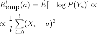
This is the risk incurred by using estimate a, estimated on a finite sample drawn from the true density. In our case it is the following


Because the sample is a random variable, empirical risk is also a random variable. We can use the method of transformations to find it's distribution. Here are distributions for empirical risk estimated from training sets of size one for different values of a.



You can see that the modes of the distributions correspond to the true risk (a^2), but the means don't.

5.

Supremum is defined as the least upper bound, and behaves lot like maximum. It is more general than the maximum however. Consider the sequence 0.9, 0.99, 0.999, ....
This sequence does not have a maximum but has a supremum.

6.

This is the simplified middle part of the equation. It represents the probability of our empirical risk underestimating true risk by more than epsilon, for a given value of a. This would be used in place of the supremum if we cared about pointwise as opposed to uniform, convergence. Intuitively, we expect this probability to get smaller for any fixed epsilon as the sample size l gets larger. Here are a few densities of risk distribution for a=4 and different values of l



7.

This is the random variable that represents the largest deviation of the empirical risk from corresponding true risk, over all models a. It's like an order statistic, except the samples are not IID, and there are infinitely many of them.

Questions:

• How can one find the distribution of \sup(R(a)-R_emp(a) in the setting above?
  

I came across an interesting article by Zhu and Lu talking about how non-informative priors can often be counter-intuitive. For instance suppose we are estimating parameter of a Bernoulli distribution. If we don't know anything, the most intuitive prior to use is uniform. However Jeffreys' "uninformative" prior doesn't look uniform at all:

NIPS pre-prints

A google search reveals the following preprints associated with NIPS 2005:

• Lafferty, Blei, Correlated Topic Models
  
• Lafferty, Wasserman, Rodeo - Sparse Nonparametric Regression in High Dimensions
  
• Tong Zhang and Rie K. Ando. Analysis of Spectral Kernel Design based Semi-supervised Learning.
  
• Philipp Häfliger, et al, AER Building Blocks for Multi-Layer Multi-Chip Neuromorphic Vision Systems
• Paninski, L. - Inferring prior probabilities from Bayes-optimal behavior
  
• Ahrens, M., Huys, Q. & Paninski, L.. Large-scale biophysical parameter estimation in single neurons via constrained linear regression
  
• Jack M. Wang, David J. Fleet, Aaron Hertzmann. Gaussian Process Dynamical Models.
  J.-P. Vert, R. Thurman and W. S. Noble, "Kernels for gene regulatory regions",
  
• Firas Hamze and Nando de Freitas. Hot Coupling: A Particle Approach to Inference and Normalization on Pairwise Undirected Graphs
  
• Jason E. Holt, On the Job Training
  
• Marco Cuturi, Kenji Fukumizu - Multiresolution Kernels
  
• Fan Li, Yiming Yang, Eric P. Xing. From lasso regression to feature vector machine.
  
• Jian Zhang, Zoubin Ghahramani and Yiming Yang. Learning Multiple Related Tasks using Latent Independent Component Analysis.
  
• James Diebel, An Application of Markov Random Fields to Range Sensing
  
• A Computational Model of Eye Movements during Object Class Detection, Wei Zhang, Dimitris Samaras, Hyejin Yang, Greg Zelinsky
  
• Cue Integration in Figure/Ground Labeling Xiaofeng Ren, Charless Fowlkes
  
• Nelson, JD; Cottrell, GW; Filimon, F; Sejnowski, T (2005, Dec). Optimal experimental design models of naive human information acquisition. NIPS 2005
  
• W. Zhang, D. Samaras, H. Yang and G. Zelinsky. A Computational Model of Eye Movements during Object Class Detection
  
• Peter Gehler and max Welling Products of "Edge-Perts"
  
• Cesa-Bianchi, Improved risk tail bounds for on-line algorithms
  
• Semi-supervised Learning with Penalized Probabilistic Clustering. NIPS 2005 Zhengdong Lu, Todd Leen
  
• LeCun, et al - Off-Road Obstacle Avoidance through End-to-End Learning
  
• Sparse Covariance Selection via Robust Maximum Likelihood Estimation Authors: Onureena Banerjee, Alexandre d'Aspremont, Laurent El Ghaoui
  
• Glenn Fung, Romer Rosales, Balaji Krishnapuram - Learning Rankings via Convex Hull Separations
  
• Maximum Margin Semi-Supervised Learning for Structured Variables - Y. Altun, D. McAllester, M. Belkin
  
• A Domain Decomposition Method for Fast Manifold Learning. Zhenyue Zhang and Hongyuan Zha
  
• C. Scott and R. Nowak, ``Learning Minimum Volume Sets,"
  
• huys qjm / zemel r / natarajan r / dayan pm - fast population coding
  
• Two view learning: SVM-2K, Theory and Practice" by Jason D. R. Farquhar, David R. Hardoon, Hongying Meng, John Shawe-Taylor and Sandor Szedmak
  
• N. Loeff and A.Sorokin and H. Arora and D.A. Forsyth, ``Efficient Unsupervised Learning for Localization and Detection in Object Categories'', NIPS 2005
  
• T. Roos, , P. Grünwald, P. Myllymäki and H.Tirri. Generalization to Unseen Case
  
• Mooy, J., & Kappen, H.J. Validity estimates for loopy belief propagation on binary real-world networks
  
• Jorge G. Silva, Jorge S. Marques, João M. Lemos, Selecting Landmarkpoints for Sparse manifold Learning
  
• Fleuret, F. and Blanchard, G. - Pattern Recognition from One Example by Chopping
  
• A Probabilistic Approach for Optimizing Spectral Clustering - R. Jin ,C.Ding and F.Kang
  
• Keiji Miura, Masato Okada, Shun-ichi Amari - Unbiased Estimator of Shape Parameter for Spiking Irregularities under Changing Environments
  
• Blatt D. and Hero A. O., "From weighted classification to policy search"
  
• A Connectionist Model for Constructive Modal Reasoning. A.d'Avila Garcez. Luis C. Lamb and Dov Gabbay
  
• J. Ting, A. D'Souza, K. Yamamoto, T. Yoshioka, D. Hoffman, S. Kakei, L. Sergio, J. Kalaska, M. Kawato, P. Strick and S. Schaal. Predicting EMG Data from M1 Neurons with Variational Bayesian Least Squares.
  
• G. L. Li, T.-Y. Leong, Learning Causal Bayesian Network with Constraints from Domain Knowledge
  
• G. L. Li, T.-Y. Leong, Learning Bayesian Networks with Variable Grouping Methods.
  
• L. Itti and P. Baldi. "Bayesian Surprise Attracts Human Attention"
  
• Q-Clustering M. Narasimhan, N. Jojic and J. Bilmes
  
• Nando de Freitas, Yang Wang, Maryam Mahdaviani, Dustin Lang. Fast Krylov Methods for N-Body Learning.
  
• Consistency of One-Class SVM and Related Algorithms, R. Vert and J.-P. Vert
  
• A. J. Bell and L. C. Parra, "Maximising sensitivity in a spiking network,"
  
• R. S. Zemel, Q. J. M. Huys, R. Natarajan, and P. Dayan, "Probabilistic computation
  
• in spiking populations," in Advances in NIPS, 2005
  
• C. Yang, R. Duraiswami and L. Davis: "Efficient Kernel Machines Using the Improved Fast Gauss Transform", NIPS 2005
  
• F. Orabona. Object-based Model of the Visual Attention for Imitation
  
• Jieping Ye, Ravi Janardan, Qi Li. Two-Dimensional Linear Discriminant Analysis
  
• L. Song, E. Gordon, and E. Gysels, "Phase Synchrony Rates for the Recognition of Motor Imageries in BCIs"
  
• Kakade, S., M. Seeger and D. Foster: Worst-Case Bounds for Gaussian Process Models.
  
• Shen, Y., A. Ng and M. Seeger: Fast Gaussian Process Regression using KD-Trees.
  
• Kevin J. Lang - Fixing two weakness of the Spectral Method
  
• Kari Torkkola and Eugene Tuv. Ecumenical kernels from random forests
  
• C. Molter and U. Salihoglu and H. Bersini, Storing information through complex dynamics in Recurrent Neural Networks
  
• J. Ting, A. D'Souza, K. Yamamoto, T. Yoshioka, D. Hoffman, S. Kakei, L. Sergio, J. Kalaska, M. Kawato, P. Strick and S. Schaal. Predicting EMG Data from M1 Neurons with Variational Bayesian Least Squares
  
• Z. Nenadic, D.S. Rizzuto, R.A. Andersen, and J.W. Burdick, "Discriminat basedfeature selection with information theoretic objective
  
• Mooy, J., & Kappen, H.J. (2004). Validity estimates for loopy belief propagation on binary real-world networks
  
• Lackey, J. and Colagrosso, M (2005). A Kernel Method for Polychotomous Classification
  
• J. A. Palmer, K. Kreutz-Delgado, D. P. Wipf, and B. D. Rao, Variational EM Algorithms for Non-Gaussian Latent Variable Models
  
• Singh, S., Barto, A., and Chentanez, N. (2005). Intrinsically motivated reinforcement learning
  
• Yun-Gang Zhang, Changshui Zhang, Separation of Music Signals by Harmonic Structure Modeling.
  
• Rob Powers, Yoav Shoham, New Criteria and a New Algorithm for Learning in Multi-Agent Systems
  
• Wood, F., Roth, S., and Black, M. J., "Modeling neural population spiking activity with Gibbs distributions,
  
• Hinton, G. E. and Nair, V. Inferring motor programs from images of handwritten digits.
  
• Onureena Banerjee, Alexandre d'Aspremont, Laurent El Ghaoui - Sparse Covariance Selection via Robust Maximum Likelihood Estimation.
  
• "Measuring Shared Information and Coordinated Activity in Neuronal Networks." K. Klinkner, C. Shalizi, and M. Camperi, NIPS, 2005.
  
• Generalisation Error Bounds for Classifiers Trained with Interdependent Data Usunier N., Amini M.-R., Gallinari P
  
• Brafman, R. I. and Shani, G. "Resolving perceptual asliasing with noisy sensors"
  
• Griffiths, T.L., and Ghahramani, Z. (to appear) Infinite Latent Feature Models and the Indian Buffet Process
  
• Zhang, J., Ghahramani, Z. and Yang, Y. (to appear) Learning Multiple Related Tasks using Latent Independent Component Analysis.
  
• Murray, I., MacKay, D.J.C., Ghahramani, Z. and Skilling, J. (to appear) Nested Sampling for Potts Models.
  
• Snelson, E. and Ghahramani, Z. (to appear) Sparse Parametric Gaussian Processes
  
• Ghahramani, Z. and Heller, K.A. (to appear) Bayesian Sets
  
• On the Convergence of Eigenspaces in Kernel Principal Component Analysis: G. Blanchard and L. Zwald
  
• Poupart, P. and Boutilier, C. VDCBPI: an Approximate Scalable Algorithm for Large Scale POMDPs
  
• T. Murayama and P. Davis, Rate distortion codes for sensor networks: A system-level analysis,
  
• Damian Eads, Karen Glocer, Simon Perkins, and James Theiler (2005). Grammar-guided feature extraction for time series classification.
  
• Doi, E., Balcan, D. C., & Lewicki, M. S. A theoretical analysis of robust coding over noisy overcomplete channels
  
• Nadler, Boaz; Lafon, Stephane; Coifman, Ronald R.; Kevrekidis, Ioannis G. - Diffusion Maps, Spectral Clustering and Eigenfunctions of Fokker-Planck operators
  
• "Abstractions and Hierarchies for Learning and Planning" Lihong Li
  
• "Walk-sum interpretation and analysis of Gaussian belief propagation ," Jason K. Johnson, Dmitry M. Malioutov, and Alan S. Willsky
  
• Baker C., Tenenbaum J., & Saxe R. - Bayesian models of perceiving.intentional action
  
• Tensor Subspace Analysis - Xiaofei He, Deng Cai, and Partha Niyogi
  
• Laplacian Score for Feature Selection - Xiaofei He, Deng Cai, and Partha Niyogi.
  
• Shunji Satoh ``Long-Range Horizontal Connections in V1 Serve to Multi-Scale Image Reconstruction
  
• "Faster Rates in Regression via Active Learning" Rebecca Willett with R. Castro and R. Nowak,
  
• Hyperparameter and Kernel Learning for Graph Based Semi-Supervised Classification - Ashish Kapoor, Yuan (Alan) Qi, Hyungil Ahn and Rosalind W. Picard
  
• Maxim Raginsky, Svetlana Lazebnik - Estimation of intrinsic dimensionality using high-rate vector quantization
  
• Ofer Dekel, Shai Shalev-Shwartz, Yoram Singer - The Forgetron: A Kernel-Based Perceptron on a Fixed Budget
  
• Patrick Flaherty, Michael Jordan, Adam Arkin - Robust Design of Biological Experiments
  
• Yael Niv, Nathaniel Daw, Peter Dayan - How Fast to Work: Response Vigor, Motivation and Tonic Dopamine
  
• Learning from Data of Variable Quality - Koby Crammer, Michael Kearns, and Jennifer Wortman
  
• R. Kondor and T. Jebara - Gaussian and Wishart Hyperkernels
  
• L. Liao, D. Fox, and H. Kautz. - Location-Based Activity Recognition Reinforcement Learning of Local Shape in the Game of Atari-Go David Silver, Richard Sutton, Martin Müller, Markus Enzenberger