Fast convergence would also imply minimum of Bethe free energy approximation to be a good approximation to true free energy (we know that BP fixed points are local minima of Bethe free energy, and also that fast convergence implies fixed points are close together), which means that Bethe free energy approximations are good
We can restrict ourselves to 1 dimensional binary chain model with constant local potentials/evidence
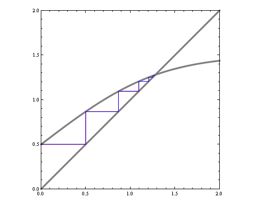
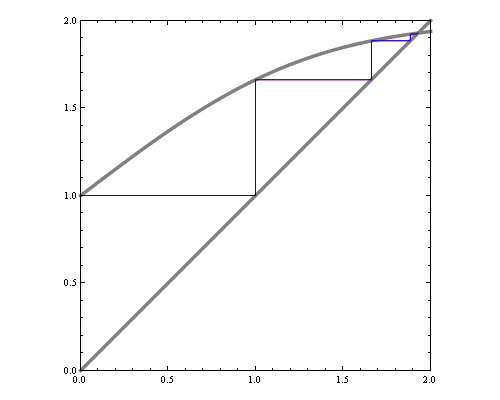
One way to visualize fixed point iteration is through a cob-web plot. Each iteration can be viewed as a horizontal projection to y=x line, then vertical projection to the curve. For instance, here are fixed point iterations for the BP equations of 1d Ising model (equivalent to 2-state hidden markov chain) for weak and strong local potentials.
If we'd like to see how the number of iterations till convergence depends on magnetic field and interaction parameters, we could try approximate the function with a quadratic around fixed point, and compute the number of fixed point iterations needed for that quadratic. However, that by itself is a hard problem. Consider fixed point iterations of the quadratics below
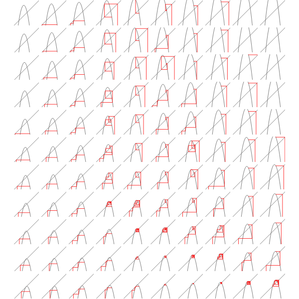
We can replace each plot in the image above by a point that's colored according to how many fixed point iterations were required to converge, keeping same scale but adding some intermediate points we get the diagram below.

You can see the tell-tale signs of chaos in the diagram above, so clearly the general problem of finding convergence rate of fixed point iterations for quadratics is hard.
We can do an analogous plot for the iterations of original BP equation
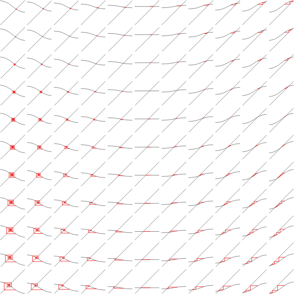
And similarly coloring the points according to the number of iterations needed to converge we get:
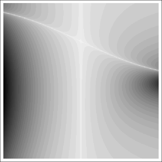
x axis here shows interaction strength between neighbours. You can see with 0 interaction, BP converges in 1 step. Y axis is the strength of evidence. You can see the slowest convergence speed is when there's strong negative corellation between neighbours, or when there's strong positive corellation, and strong negative local evidence. The plot is lopsided because my initial point was 0.5.
This doesn't exhibit the chaotic structure, so in this case reducing the problem to general quadratic actually makes the problem harder.
Mathematica notebook
9 comments:
I really amazed to have this wonderful post
anal dildo
Excellent machine learning blog,thanks for sharing...
Seo Internship in Bangalore
Smo Internship in Bangalore
Digital Marketing Internship Program in Bangalore
This looks oddly satisfying, I was watching it on TikTok to Mp4
Great looking web site. Assume you did a lot of your very own html coding.
The Provided information on you blog is too good.
It’s awesome that you want to share those tips with us.
I want to always read your blogs.
I really enjoyed this blog post, thank you for sharing it.
Thanks for posting this, it was unbelievably informative and helped me a lot
Post a Comment