- Scalable Training of L1-regularized Log-linear ModelsThe main idea is to do L-BFGS in an orthant where the gradient of the L1 loss doesn't change. Each time BFGS tries to step out of that orthant, project it's new point on the old orthant, and figure out the new orthant to explore
- Discriminative Learning for Differing Training and Test DistributionsIn addition to learning P(Y|X,t1), also learn P(this point is from test data|X). You can do logistic regression to model P(this point is from test data|X,t2), and then weight each point in training set by that value when learning P(Y|X). Alternatively you can learn both distributions simultaneously by maximizing P(Y|X,t1,t2) on test data, which gives even better results
- On One Method of Non-Diagonal Regularization in Sparse Bayesian Learning Relevance Vector Machine "fits" a diagonal Gaussian prior to data by maximizing P(data|prior).
In the paper they get a tractable method of fitting Laplace/Gaussian priors with non-diagonal matrices by first transforming parameters to a basis which uncorrelates the parameters at the point of maximum likelihood. - Piecewise Pseudolikelihood for Efficient Training of Conditional Random FieldsDoing pseudo-likelihood training (replacing p(y1,y2|x) with p(y1|y2,x)p(y2|y1,x)) on small pieces of the graph (piece-wise training) gives better accuracy than pseudo-likelihood training on the true graph
- CarpeDiem: an Algorithm for the Fast Evaluation of SSL Classifiers -- a useful trick for doing Viterbi faster -- don't bother computing forward values for nodes which are certain to not be included in the best path. You know a node will not be included in the search path if the a+b+c is smaller than some other forward value on the same level. a+b+c is largest forward value on previous level, b is largest possible transition weight, c is the "emission" weight for that node
Thursday, June 28, 2007
Cool Papers at ICML 07
Here are a few that caught my eye:
Wednesday, June 27, 2007
Machine Learning patents
I found a large number of machine learning related patent applications by doing a few queries on http://www.freepatentsonline.com/
Here are a couple that caught my eye:
The interesting question is what the companies will do with those patents. The best thing they can do is to do nothing with them, which seems to be the case for most patents. The worst thing is they can go after regular users that make implementations of those methods freely available. For instance Xerox forced someone I know to remove a visualization applet from their webpage because the applet used hyperbolic space to visualize graphs, and they have patented this method of visualization. Here are some more worst-case scenarios
Does anyone have any other examples of notable machine learning patents/applications?
Here are a couple that caught my eye:
- Logistic regression (A machine implemented system that facilitates maximizing probabilities)
- Boosting (A computer-implemented process for using feature selection to obtain a strong classifier from a combination of weak classifiers)
- Decision tree? (Machine learning by construction of a decision function)
- Bayesian Conditional Random Fields -- notably, Tom Minka is missing from the list of inventors
The interesting question is what the companies will do with those patents. The best thing they can do is to do nothing with them, which seems to be the case for most patents. The worst thing is they can go after regular users that make implementations of those methods freely available. For instance Xerox forced someone I know to remove a visualization applet from their webpage because the applet used hyperbolic space to visualize graphs, and they have patented this method of visualization. Here are some more worst-case scenarios
Does anyone have any other examples of notable machine learning patents/applications?
Tuesday, June 12, 2007
Log loss or hinge loss?
Suppose you want to predict binary y given x. You fit a conditional probability model to data and form a classifier by thresholding on 0.5. How should you fit that distribution?
Traditionally people do it by minimizing log-loss on data, which is equivalent to maximum likelihood estimation, but that has the property of recovering the conditional distribution exactly with enough data/modelling freedom. We don't care about exact probabilities, so in some sense it's doing too much work.
Additionally, log-loss minimization may sacrifice classification accuracy if it allows it to model probabilities better.
Here's an example, consider predicting binary y from real valued x. The 4 points give the possible 4 possible x values and their true probabilities. If you model p(y=1|x) as 1/(1+Exp(f_n(x))) where f_n is any n'th degree polynomial.
Take n=2, then minimizing log loss and thresholding on 1/2 produces Bayes-optimal classifier
However, for n=3, the model that minimizes log loss will have suboptimal decision rules for half the data.
Hinge loss is less sensitive to exact probabilities. In particular, minimizer of hinge loss over probability densities will be a function that returns returns 1 over the region where true p(y=1|x) is greater than 0.5, and 0 otherwise. If we are fitting functions of the form above, then once hinge-loss minimizer attains the minimum, adding extra degrees of freedom will never increase approximation error.
Here's example suggested by Olivier Bousquet, suppose your decision boundaries are simple, but the actual probabilities are complicated, how well will hinge loss vs log loss do? Consider the following conditional density
Now use the conditional density functions of the same form as before, find minimizers of both log-loss and hinge loss. Hinge-loss minimization always produces Bayes optimal model for all n>1
When minimizing log-loss, the approximation error starts to increase as the fitter tries to match the exact oscillations in the true probability density function, and ends up overshooting.
Here's the plot of the area on which log loss minimizer produces suboptimal decision rule
Mathematica notebook (web version)
Thursday, May 03, 2007
Mathematica 6.0 is out
Mathematica 6.0 is out, touted "The most important advance in the 20-year history of Mathematica"
Among the highly anticipated features is the support for joysticks/gamepads (an XBox version is surely to follow shortly), and the ability to use freehand doodles instead of mathematical symbols in equations (handy when you run out of latin/greek alphabets in your equations)
Among the highly anticipated features is the support for joysticks/gamepads (an XBox version is surely to follow shortly), and the ability to use freehand doodles instead of mathematical symbols in equations (handy when you run out of latin/greek alphabets in your equations)
Thursday, May 18, 2006
Curse of Dimensionality and intuition
There are some counter-intuitive things happening as dimension increases.
For instance consider unit sphere (radius 1)
If you go from 2 dimensions to 3 dimensions, the volume increases (Pi to 4/3 pi). Similar increase happens when you go to 3,4,5 dimensions. But then the volume starts to decrease. Eventually it decreases all the way to 0.
Now consider a cube of width 1. As dimension increases, the volume stays the same. But the length of the main diagonal grows as sqrt(dimension). So the corners become situated further and further away from the center, and eventually almost all the mass is concentrated in the corners (meaning outside of the inscribed sphere)
Here's a plot of the fraction of the mass concentrated in the corners as a function of dimension
For a 7 dimensional cube, about 96% of the mass is concentrated in one of it's 128 "corners", so if we had 7 dimensional vision, we might see that cube like this
Finally consider what happens with a d-dimensional standard normal (unit covariance matrix, centered at 0). If we plot probability mass contained around a thin shell of radius r as a function r we get the following graphs (d=1,d=4,d=16)
The mean of this distribution is
which can be approximated as sqrt(d)
Furthermore you can derive that variance of this distribution converges to 1/2 (see notebook). Applying Chebyshev's inequality, we get that for any dimension, at least 0.75 of the mass is contained in the shell of thickness 1 centered at about sqrt(d). In numerical integration this seems to converge to a slightly higher number, for instance for 10^6 dimensions, it's about 0.84
Here's the Mathematica notebook with some derivations (web version)
Tuesday, May 09, 2006
Positive-definite/negative-definite
Concepts of positive definite matrices and positive definite operators often come up in Machine Learning, here are some movies I made to visualize linear transformations corresponding to some common types of matrices:
Symmetric and positive definite
Symmetric positive definite matrices can be thought of matrices that stretch or shrink the circle along the eigenvectors (marked in blue).
The angle between x and Ax is always less than Pi/2, so x'Ax>0 forall x.
Symmetric and negative definite
You can see in addition to stretching, every vector is flipped across the origin. So the angle is always between Pi/2 and Pi, hence x'Ax<0>0 and for others x'Ax
Symmetric and indefinite
Vectors are flipped across one axis only, so sometimes the angle is more than Pi/2 and sometimes it's less. A quadratic form corresponding to such matrix will have a saddle point (you can see this because x'Ax will be positive along some directions, and negative along others)
Positive definite but not symmetric
Rotation by less than Pi/2 and positive skew are positive definite operations, even though they are not symmetric or diagonalizable.
You can see in the first case there's only one vector (0,1) that does't change direction after action by A, so there's only 1 eigenvector, hence the matrix is not diagonalizable. In the second case, every vector changes after action by A so there are no (real) eigenvectors, and matrix is again not diagonalizable.
Saturday, April 29, 2006
Naive Bayes vs. Logistic Regression
There's often confusion as to the nature of the differences between Logistic Regression and Naive Bayes Classifier. One way to look at it is that Logistic Regression and NBC consider the same hypothesis space, but use different loss functions, which leads to different models for some datasets.
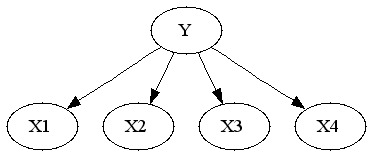
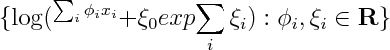
To see that both logistic regression and naive bayes classifier consider the same hypothesis space we can rewrite Naive Bayes density as follows (restricting attention to binary domain):

where
Alternatively you can get exponential family parametrization from the observation that Naive Bayes model has no unshielded colliders, so undirected model obtained by dropping the arrows is equivalent on the set of positive densities.
From here you can rewrite it as product of conditional and marginal distributions
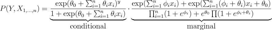
You can see that the conditional term is equivalent to logistic regression, so every possible conditional density that can be modelled by logistic regression can be modelled by Naive Bayes by setting \phi's aribrarily.
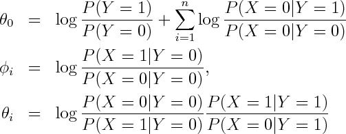
So both logistic regression and Naive Bayes have the same hypothesis space, but optimize different objective functions. In particular logistic regression maximizes
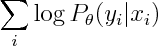
whereas Naive Bayes maximizies
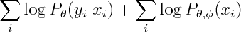
You can see that the second term involves both phis and thetas, so conditional and marginal likelihoods are coupled. If empirical density is realizable by our model, then this coupling doesn't matter -- both conditional and marginal terms can achieve their respective maxima so Naive Bayes and Logistic Regression will produce the same estimate. However that not necessarily true when empirical density is unrealizable -- you may have to compromise between achieving high conditional likelihood and high marginal likelihood.
To get a generatively trained model that is identical to conditionally trained Naive Bayes, Minka suggests treating parameters in conditional and joint as separate sets.
So now we can introduce n new parameters so that conditional and marginal densities become decoupled.

It's interesting to see what is the new marginal density of our model. The marginal density marginalizes out Y. Since Y is the only separator in original graph, the resulting graph will be fully connected.
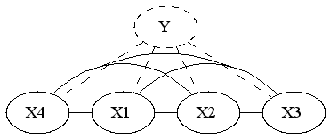
So if we were to restrict attention to linear exponential families, we'd have to introduce 2^n features. I'm wondering if it's possible to infer that fact by looking at the form of the density. You'd have to show that the size of sufficient statistic is at least 2^n, or alternatively show that the smallest linear space that embeds the unnormalized log densities has dimension 2^n
If x_i are real or complex valued, one could show that the smallest linear space that embeds the set above has to be infinite dimensional, by noting that since log(1+exp(ax)) has singularities at i pi a, so one can always construct linearly independent elements by choosing a accordingly. I wonder, are there similar tricks that would work for discrete x?
(derivations)
To see that both logistic regression and naive bayes classifier consider the same hypothesis space we can rewrite Naive Bayes density as follows (restricting attention to binary domain):
where
Alternatively you can get exponential family parametrization from the observation that Naive Bayes model has no unshielded colliders, so undirected model obtained by dropping the arrows is equivalent on the set of positive densities.
From here you can rewrite it as product of conditional and marginal distributions
You can see that the conditional term is equivalent to logistic regression, so every possible conditional density that can be modelled by logistic regression can be modelled by Naive Bayes by setting \phi's aribrarily.
So both logistic regression and Naive Bayes have the same hypothesis space, but optimize different objective functions. In particular logistic regression maximizes
whereas Naive Bayes maximizies
You can see that the second term involves both phis and thetas, so conditional and marginal likelihoods are coupled. If empirical density is realizable by our model, then this coupling doesn't matter -- both conditional and marginal terms can achieve their respective maxima so Naive Bayes and Logistic Regression will produce the same estimate. However that not necessarily true when empirical density is unrealizable -- you may have to compromise between achieving high conditional likelihood and high marginal likelihood.
To get a generatively trained model that is identical to conditionally trained Naive Bayes, Minka suggests treating parameters in conditional and joint as separate sets.
So now we can introduce n new parameters so that conditional and marginal densities become decoupled.
It's interesting to see what is the new marginal density of our model. The marginal density marginalizes out Y. Since Y is the only separator in original graph, the resulting graph will be fully connected.
So if we were to restrict attention to linear exponential families, we'd have to introduce 2^n features. I'm wondering if it's possible to infer that fact by looking at the form of the density. You'd have to show that the size of sufficient statistic is at least 2^n, or alternatively show that the smallest linear space that embeds the unnormalized log densities has dimension 2^n
If x_i are real or complex valued, one could show that the smallest linear space that embeds the set above has to be infinite dimensional, by noting that since log(1+exp(ax)) has singularities at i pi a, so one can always construct linearly independent elements by choosing a accordingly. I wonder, are there similar tricks that would work for discrete x?
(derivations)
Monday, April 17, 2006
Derivation of probability calculus
Here is an succinct derivation of probability calculus by Skillings (appeared in Appendix of his MaxEnt 2005 "Bayesics" article)
Friday, March 31, 2006
Graphical Models class notes
I needed to refresh some Graphical Models basics, and here are lecture notes I found useful
- Jeff Bilmes' Graphical Models course , gives detailed introduction on Lauritzen's results, proof of Hammersley-Clifford results (look in "old scribes" section for notes)
- Kevin Murphy's Graphical Models course , good description of I-maps
- Sam Roweis' Graphical Models course , good introduction on exponential families
- Stephen Wainwright's Graphical Models class, exponential families, variational derivation of inference
- Michael Jordan's Graphical Models course, his book seems to be the most popular for this type of class
- Lauritzen's Graphical Models and Inference class , also his Statistical Inference class , useful facts on exponential families, information on log-linear models, decomposability
- Donna Precup's class , some stuff on structure learning
Wednesday, March 22, 2006
Challenge: Online Learning for Cell Phone Messaging
 If you've used cell phones to send text messages you probably know about their auto-complete feature. For those that haven't -- each digit corresponds to 3 or 4 letters, you enter the digits consistent with your word, and it tries to guess which word you meant. For instance you enter "43556", and it will automatically guess "hello". But if you enter "785" to mean "SVM", it'll probably guess "run", and you'll have to back-up and re-enter the word. The challenge is for the phone to guess the right word.
Since new abbreviations spring up all the time, there's no dictionary that can cover all the words used in text-messages, so an ideal cell-phone will have an algorithm that can adapt to the user. The interesting question is how well can you do?
What makes this domain different from other sources of text is that it's a conversation, consisting of a series of short posts, containing colloquial grammar, bad spelling and abbreviations. I ran some simple algorithms on a similar dataset - 1.5M words of posts from a single person from an online chatroom.
The simplest algorithm is to return the most recent word encountered, consistent with given numbering. You can also return the most frequent word, or have a compound learner that returns one or the other. Cost of 1 is incurred every time an incorrect word is guessed. Here's what the curves look like

The "best rate" curve represents the cost incurred if we only make errors on words that haven't been seen before. After 1.5M words, this "algorithm" makes mistakes about 20% of the time relative to the simple learners, which means there's a lot of room for improvement. And since this "algorithm" only sees 2-3 candidates for each word entered, there's no need to worry about efficient inference.
So here's a challenge -- can you approach the "best rate" curve any closer without using any other sources of text? (like dictionaries) If so, I'd like to hear from you! Here's the simplest script to generate an evaluation like above.
(BTW, I have several GB's of chatlogs, and I'll make more data available if there's demand)
Friday, March 03, 2006
Machine Learning videos
Learning from presentation or slides can be a much easier than from papers. I was reminded of that when I ran across Martin Wainwright's excellent class on Graphical Models. It has lecture notes *and* videos online.
Another large repository of machine learning related videos is the repository organized by the Pascal Network. You may run into a couple of bugs, but Sebastjan Mislej (sebastjan dot mislej dot ijs dot si) is very quick at fixing them when you email him.
Does anyone else have a favourite set of Machine Learning slides/notes/videos online?
Friday, December 16, 2005
Trends in Machine Learning according to Google Scholar
In a previous post I brought up the 1983 Machine Learning workshop which featured "33 papers", and it was the follow up to the 1980 Machine Learning workshop. By contrast, NIPS 2005 had 28 workshops and is just one of several international annual Machine Learning Conferences. You can see how the field grew by looking at the distribution of publication dates for articles containing phrase "machine learning" indexed by Google Scholar (normalized by total Scholar content for each year)
You can see there's a blip at 1983 when the workshop was held.
Yann LeCun quipped at NIPS closing banquet that people who joined the field in the last 5 years probably never heard of the word "Neural Network". Similar search (normalized by results for "machine learning") reveals a recent downward trend.
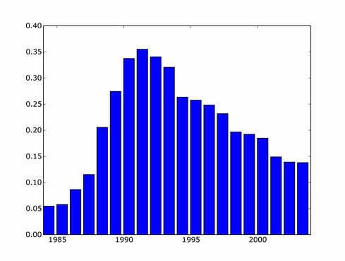
You can see a major upward trend starting around 1985 (that's when Yann LeCun and several others independently rediscovered backpropagation algorithm), peaking in 1992, and going downwards from then.
An even greater downward trend is seen when searching for "Expert System",

"Genetic algorithms" seem to have taken off in the 90's, and leveled off somewhat in recent years

On other hand, search for "support vector machine" shows no sign of slowing down

(1995 is when Vapnik and Cortez proposed the algorithm)
Also, "Naive Bayes" seems to be growing without bound

If I were to trust this, I would say that Naive Bayes research the hottest machine learning area right now
"HMM"'s seem to have been losing in share since 1981

(or perhaps people are becoming less likely to write things like "hmm, this result was unexpected"?)
What was the catastrophic even of 1981 that forced such a rapid extinction of HMM's (or hmm's) in scientific literature?
Finally a worrying trend is seen in the search for "artificial stupidity" divided by corresponding hits for "artificial intelligence". The 2000 through 2004 graph shows a definite updward direction.

You can see there's a blip at 1983 when the workshop was held.
Yann LeCun quipped at NIPS closing banquet that people who joined the field in the last 5 years probably never heard of the word "Neural Network". Similar search (normalized by results for "machine learning") reveals a recent downward trend.
You can see a major upward trend starting around 1985 (that's when Yann LeCun and several others independently rediscovered backpropagation algorithm), peaking in 1992, and going downwards from then.
An even greater downward trend is seen when searching for "Expert System",
"Genetic algorithms" seem to have taken off in the 90's, and leveled off somewhat in recent years
On other hand, search for "support vector machine" shows no sign of slowing down
(1995 is when Vapnik and Cortez proposed the algorithm)
Also, "Naive Bayes" seems to be growing without bound
If I were to trust this, I would say that Naive Bayes research the hottest machine learning area right now
"HMM"'s seem to have been losing in share since 1981
(or perhaps people are becoming less likely to write things like "hmm, this result was unexpected"?)
What was the catastrophic even of 1981 that forced such a rapid extinction of HMM's (or hmm's) in scientific literature?
Finally a worrying trend is seen in the search for "artificial stupidity" divided by corresponding hits for "artificial intelligence". The 2000 through 2004 graph shows a definite updward direction.
Tuesday, December 13, 2005
pigeon-level AI
At the NIPS "Towards Human-Level AI" workshop one of the messages was that perhaps we should first try to achieve rat-level AI, and go from there.
But maybe instead we should start by achieving pigeon-level AI. Someone has already measured pigeon performance at discriminating between painting styles
But maybe instead we should start by achieving pigeon-level AI. Someone has already measured pigeon performance at discriminating between painting styles
Monday, December 12, 2005
Archaeology
Here's what Aleks Jakulin managed to dig up in Google newsgroup archives
"1983 INTERNATIONAL MACHINE LEARNING WORKSHOP: AN INFORMAL REPORT"
link
Some snippets
Here's Tom Dietterich again: ``I was surprised that you summarized the workshop
in terms of an "incremental" theme. I don't think incremental-ness
is particularly important--especially for expert system work.
"So the language analysis problem has been solved?!?" by Fernando Pereira, Aug 20 1983
link
" What this replacement does to modularity, testability and
reproducibility of results is sadly clear in the large amount of
published "research" in natural language analysis which is untestable
and irreproducible."
Saturday, November 12, 2005
The Key Theorem of the Learning Theory
The Key Theorem of the Learning Theory is what Vapnik calls his theorem (for instance here) that gives the necessary conditions for the Empirical Risk Minimization principle to be consistent.
The important equation is the following:
Here I'll explain the parts of the formula using the following motivating example:
Suppose our true distribution is a normal distribution with unit variance, centered at 0, and we estimate its mean from data using method of maximum likelihood. This falls into domain of Empirical Risk Minimization because it's equivalent to finding unit variance normal distribution which minimizes empirical log-loss. If this method is consistent, then our maximum likelihood estimate of the mean will be correct in the limit
In order for the theorem to apply, we need to do make sure that we can put a bound on the loss incurred by functions in our hypothesis space, so here, make an additional restriction that our fitted normals must have mean between -100 and 100.
Here's what parts of the equation stand for
1.
l is the size of our training set
2.
a is the parameter that indexes our probability distributions, in this case, it's mean of our fitted Normal. Lambda is it's domain, in this case,
3.
This is the actual risk incurred by using estimate a instead of true estimate (0). In our case the loss is log loss, so the risk is

In other words it is the expected value of the negative logarithm of the probability assigned to observations when observations come from Normal centered at 0, but we think they come from Normal centered on a
4.
This is the risk incurred by using estimate a, estimated on a finite sample drawn from the true density. In our case it is the following
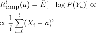
Because the sample is a random variable, empirical risk is also a random variable. We can use the method of transformations to find it's distribution. Here are distributions for empirical risk estimated from training sets of size one for different values of a.
You can see that the modes of the distributions correspond to the true risk (a^2), but the means don't.
5.
Supremum is defined as the least upper bound, and behaves lot like maximum. It is more general than the maximum however. Consider the sequence 0.9, 0.99, 0.999, ....
This sequence does not have a maximum but has a supremum.
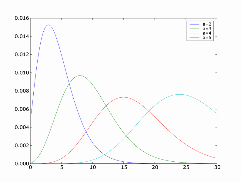
6.
This is the simplified middle part of the equation. It represents the probability of our empirical risk underestimating true risk by more than epsilon, for a given value of a. This would be used in place of the supremum if we cared about pointwise as opposed to uniform, convergence. Intuitively, we expect this probability to get smaller for any fixed epsilon as the sample size l gets larger. Here are a few densities of risk distribution for a=4 and different values of l
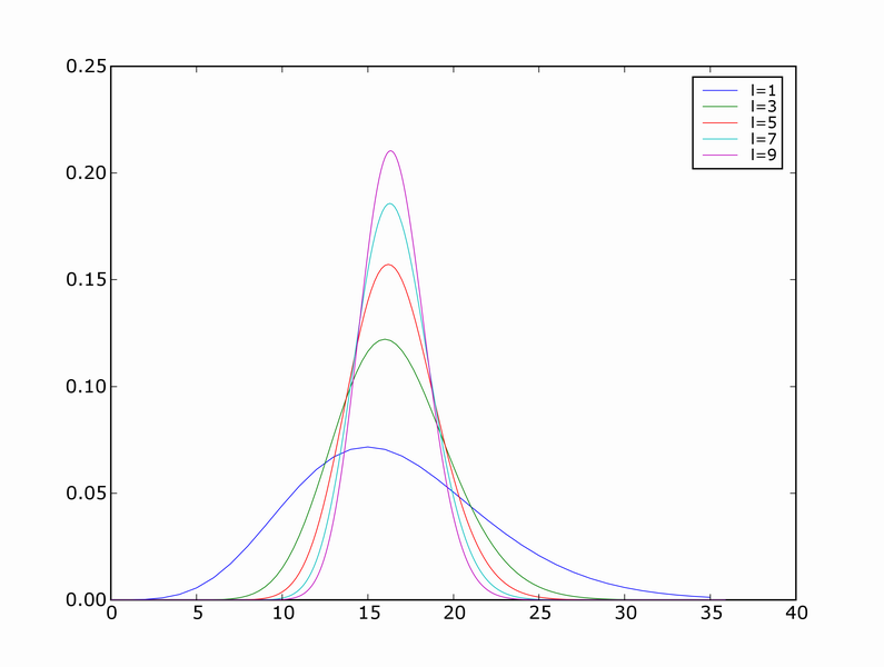
7.
This is the random variable that represents the largest deviation of the empirical risk from corresponding true risk, over all models a. It's like an order statistic, except the samples are not IID, and there are infinitely many of them.
Questions:
The important equation is the following:
Here I'll explain the parts of the formula using the following motivating example:
Suppose our true distribution is a normal distribution with unit variance, centered at 0, and we estimate its mean from data using method of maximum likelihood. This falls into domain of Empirical Risk Minimization because it's equivalent to finding unit variance normal distribution which minimizes empirical log-loss. If this method is consistent, then our maximum likelihood estimate of the mean will be correct in the limit
In order for the theorem to apply, we need to do make sure that we can put a bound on the loss incurred by functions in our hypothesis space, so here, make an additional restriction that our fitted normals must have mean between -100 and 100.
Here's what parts of the equation stand for
1.
l is the size of our training set
2.
a is the parameter that indexes our probability distributions, in this case, it's mean of our fitted Normal. Lambda is it's domain, in this case,
3.
This is the actual risk incurred by using estimate a instead of true estimate (0). In our case the loss is log loss, so the risk is
In other words it is the expected value of the negative logarithm of the probability assigned to observations when observations come from Normal centered at 0, but we think they come from Normal centered on a
4.
This is the risk incurred by using estimate a, estimated on a finite sample drawn from the true density. In our case it is the following
Because the sample is a random variable, empirical risk is also a random variable. We can use the method of transformations to find it's distribution. Here are distributions for empirical risk estimated from training sets of size one for different values of a.
You can see that the modes of the distributions correspond to the true risk (a^2), but the means don't.
5.
Supremum is defined as the least upper bound, and behaves lot like maximum. It is more general than the maximum however. Consider the sequence 0.9, 0.99, 0.999, ....
This sequence does not have a maximum but has a supremum.
6.
This is the simplified middle part of the equation. It represents the probability of our empirical risk underestimating true risk by more than epsilon, for a given value of a. This would be used in place of the supremum if we cared about pointwise as opposed to uniform, convergence. Intuitively, we expect this probability to get smaller for any fixed epsilon as the sample size l gets larger. Here are a few densities of risk distribution for a=4 and different values of l
7.
This is the random variable that represents the largest deviation of the empirical risk from corresponding true risk, over all models a. It's like an order statistic, except the samples are not IID, and there are infinitely many of them.
Questions:
- How can one find the distribution of \sup(R(a)-R_emp(a) in the setting above?
Subscribe to:
Posts (Atom)