Loopy Belief propagation

Consider a distribution over 6 binary random variables captured by the structure below.



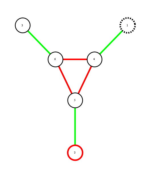
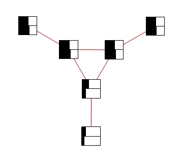
Red represents -1 potential, green represents +1 potential. More precisely, it's the diagram of the following model, where x's are {-1,1}-valued



We'd like to find the odds of x1 being 1. You could do it by dividing sum of potentials over labellings with x1=1 by corresponding sum over labellings with x1=-1.



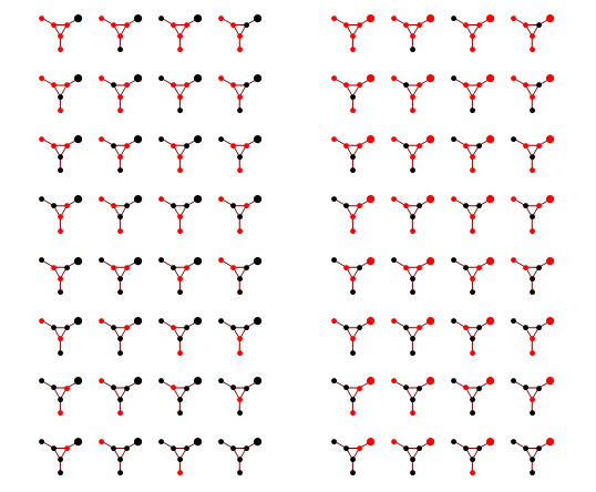
In a graph without cycles, such sums can be computed in time linear in the number of nodes by means of dynamic programming. In such cases it reduces to a series of local updates







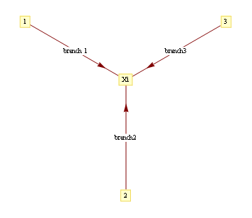
where evidence (or potential) from each branch is found by marginalizing over the separating variable



For binary states, update equations become particularly simple.



Here, m_{i,j} is the "message" being sent from node i to node j. If we view message passing as a way of computing marginal conditioned on the evidence, then message {i,j} represents the log-odds that node i is positive, given all the evidence on the other side of of the edge i,j. If our graph has loops, then "other side" of the edge doesn't make sense, but you can use the equations anyway, and this is called "loopy BP".

For binary networks with at most 1 loop, Yair Weiss showed that even though loopy BP may give incorrect probability estimates, highest probability labels under BP will be the same.

Implementation of loopy BP is below. Basically you add up all the messages from neighbours, subtract the message of the target node, then "squash" the message towards zero using ArcTanh[Tanh[J]Tanh[x]] function. Procedure loopyBP takes a matrix of connections, local potential strengths, and returns a function that represents one iteration of BP. Below you see the first few iterations for the graphical model above






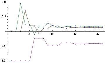
To get the final potential at any given node, just add up all the incoming messages. For the graph above, we can plot the probabilities and see that they fall on the correct side of zero after 10 iterations, so that is much smaller computational burden than exact marginalization.




Below you can see the estimates produced by running loopy BP for 200 iterations. The top bar at each node is the actual probability, the bottom bar is the estimated probability using loopy BP. You can see that the feedback makes the estimates overly confident.



For graphs with more than one cycle, loopy BP is no longer guaranteed to converge, or to give MAP labelling when it converges. For instance, here's an animation of loopy BP applied to square Ising lattice with randomly initialized neighbour potentials




Some methods like the Convex-Concave procedure and Generalized Belief Propagation improve on BP's convergence and accuracy.

Mathematica notebook used to produce these figures